Coursera吴恩达深度学习专项课程01: Neural Networks and Deep Learning 学习笔记 Week 02

Week 02 of Neural Networks and Deep Learning

Course Certificate

本文是学习 https://www.coursera.org/learn/neural-networks-deep-learning 这门课的笔记

Course Intro

Set up a machine learning problem with a neural network mindset and use vectorization to speed up your models.

Learning Objectives

---

• Build a logistic regression model structured as a shallow neural network
• Build the general architecture of a learning algorithm, including parameter initialization, cost function and gradient calculation, and optimization implementation (gradient descent)
• Implement computationally efficient and highly vectorized versions of models
• Compute derivatives for logistic regression, using a backpropagation mindset
• Use Numpy functions and Numpy matrix/vector operations
• Work with iPython Notebooks
• Implement vectorization across multiple training examples
• Explain the concept of broadcasting

[1] Logistic Regression as a Neural Network

Binary Classification

Hello, and welcome back.

In this week we’re going to go over
the basics of neural network programming.

It turns out that when you
implement a neural network there are some techniques that
are going to be really important.

For example, if you have a training
set of m training examples, you might be used to processing
the training set by having a for loop step through your m training examples.

But it turns out that when you’re
implementing a neural network, you usually want to process
your entire training set without using an explicit for loop to
loop over your entire training set.

So, you’ll see how to do that
in this week’s materials.

Another idea, when you organize
the computation of a neural network, usually you have what’s called a forward
pass or forward propagation step, followed by a backward pass or
what’s called a backward propagation step.

And so in this week’s materials,
you also get an introduction about why the computations in learning a neural
network can be organized in this forward propagation and
a separate backward propagation.

For this week’s materials I want
to convey these ideas using logistic regression in order to make
the ideas easier to understand.

But even if you’ve seen logistic
regression before, I think that there’ll be some new and interesting ideas for
you to pick up in this week’s materials.

So with that, let’s get started.

Logistic regression is an algorithm for
binary classification.

Set up the problem

So let’s start by setting up the problem.

Here’s an example of a binary
classification problem.

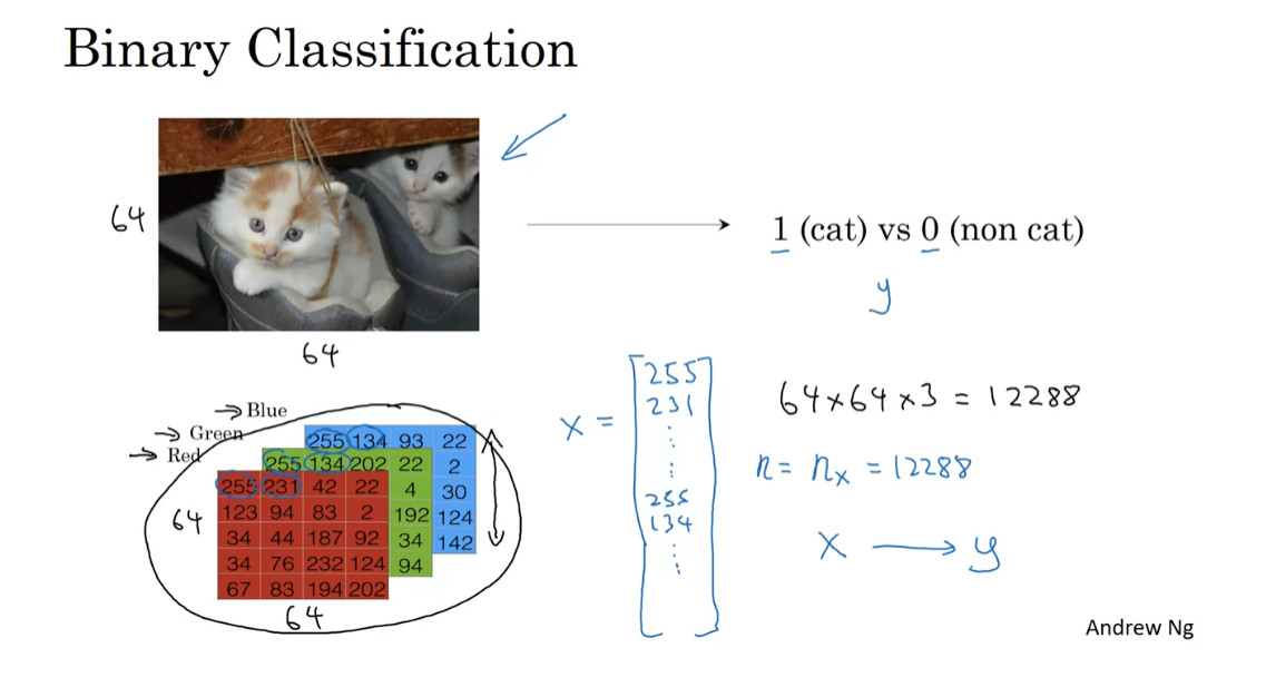
You might have an input of an image,
like that, and want to output a label to recognize
this image as either being a cat, in which case you output 1, or
not-cat in which case you output 0, and we’re going to use y
to denote the output label.

Let’s look at how an image is
represented in a computer.

To store an image your computer
stores three separate matrices corresponding to the red, green, and
blue color channels of this image.

So if your input image is
64 pixels by 64 pixels, then you would have 3 64 by 64 matrices corresponding to the red, green and blue
pixel intensity values for your images.

Although to make this little slide I
drew these as much smaller matrices, so these are actually 5 by 4
matrices rather than 64 by 64. So to turn these pixel intensity values-
Into a feature vector, what we’re going to do is unroll all of these pixel
values into an input feature vector x.

So to unroll all these pixel intensity
values into a feature vector, what we’re going to do is define a feature vector x
corresponding to this image as follows.

We’re just going to take all
the pixel values 255, 231, and so on. 255, 231, and so
on until we’ve listed all the red pixels.

And then eventually 255 134 255,
134 and so on until we get a long feature
vector listing out all the red, green and
blue pixel intensity values of this image.

If this image is a 64 by 64 image,
the total dimension of this vector x will be 64
by 64 by 3 because that’s the total numbers we have
in all of these matrixes.

Which in this case,
turns out to be 12,288, that’s what you get if you
multiply all those numbers.

And so we’re going to use nx=12288 to represent the dimension
of the input features x.

And sometimes for brevity,
I will also just use lowercase n to represent the dimension of
this input feature vector.

So in binary classification, our goal
is to learn a classifier that can input an image represented by
this feature vector x.

And predict whether
the corresponding label y is 1 or 0, that is, whether this is a cat image or
a non-cat image.

Lay out some of the notations

Let’s now lay out some of
the notation that we’ll use throughout the rest of this course.

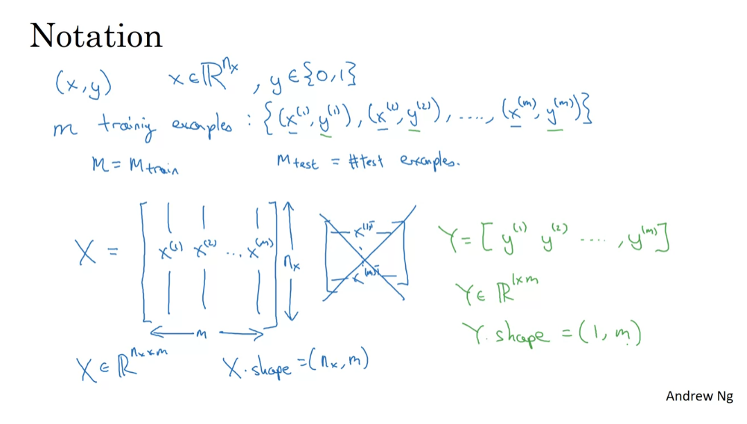
A single training example
is represented by a pair, (x,y) where x is an x-dimensional feature vector and y, the label, is either 0 or 1.

Your training sets will comprise
lower-case m training examples. And so your training sets will be
written (x1, y1) which is the input and output for your first training
example (x(2), y(2)) for the second training example up to (xm,
ym) which is your last training example.

use lowercase m to denote the number of training samples.

X is a nx by m dimensional matrix

And then that altogether is
your entire training set.

So I’m going to use lowercase m to
denote the number of training samples.

And sometimes to emphasize that this
is the number of train examples, I might write this as M = M train.

And when we talk about a test set, we might sometimes use m subscript test
to denote the number of test examples. So that’s the number of test examples.

Finally, to output all of the training
examples into a more compact notation, we’re going to define a matrix, capital X.

As defined by taking you
training set inputs x1, x2 and so on and stacking them in columns.

So we take X1 and
put that as a first column of this matrix, X2, put that as a second column and
so on down to Xm, then this is the matrix capital X. So this matrix X will have M columns,
where M is the number of train examples and the number of rows,
or the height of this matrix is NX.

Notice that in other courses,
you might see the matrix capital X defined by stacking up the train
examples in rows like so, X1 transpose down to Xm transpose.

It turns out that when you’re
implementing neural networks using this convention I have on the left,
will make the implementation much easier.

So just to recap,
X is a nx by m dimensional matrix, and when you implement this in Python, you see that x.shape,
that’s the python command for finding the shape of the matrix,
that this an nx, m.

That just means it is an nx
by m dimensional matrix.

So that’s how you group the training
examples, input x into matrix.

How about the output labels Y?

It turns out that to make your
implementation of a neural network easier, it would be convenient to
also stack Y In columns.

So we’re going to define capital
Y to be equal to Y 1, Y 2, up to Y m like so. So Y here will be a 1 by
m dimensional matrix.

And again, to use the notation
with the shape of Y will be 1, m. Which just means this is a 1 by m matrix.

And as you implement your neural network
later in this course you’ll find that a useful convention would be to take the data
associated with different training examples, and by data I mean either x or
y, or other quantities you see later.

But to take the stuff or the data associated with
different training examples and to stack them in different columns,
like we’ve done here for both x and y.

So, that’s a notation we’ll use for
a logistic regression and for neural networks networks
later in this course.

If you ever forget what a piece of
notation means, like what is M or what is N or what is something else, we’ve also posted
on the course website a notation guide that you can use to quickly look up what
any particular piece of notation means. So with that, let’s go on to the next
video where we’ll start to fetch out logistic regression using this notation.

Logistic Regression

In this video, we’ll go over
logistic regression.

This is a learning algorithm that you use
when the output labels Y in a supervised learning problem are all either zero or one, so for binary classification problems.

Given an input feature vector X
maybe corresponding to an image that you want to recognize as
either a cat picture or not a cat picture, you want an algorithm that can
output a prediction, which we’ll call Y hat, which is your estimate of Y.

what is the chance that this is a cat picture?

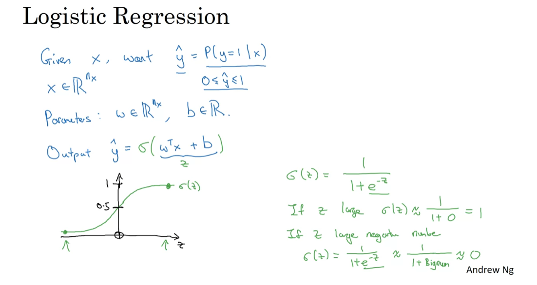
More formally, you want Y hat to be the
probability of the chance that, Y is equal to one given the input features X.

So in other words, if X is a picture, as we saw in the last video, you want Y hat to tell you, what is the chance that this is a cat picture?

So X, as we said in the previous video, is an n_x dimensional vector, given that the parameters of
logistic regression will be W which is also an
n_x dimensional vector, together with b which is just a real number.

So given an input X and the
parameters W and b, how do we generate the output Y hat?

Well, one thing you could try,
that doesn’t work, would be to have Y hat be
w transpose X plus B, kind of a linear function of the input X.

And in fact, this is what you use if
you were doing linear regression.

But this isn’t a very good algorithm
for binary classification because you want Y hat to be
the chance that Y is equal to one.

So Y hat should really be
between zero and one, and it’s difficult to enforce that
because W transpose X plus B can be much bigger than
one or it can even be negative, which doesn’t make sense for probability. That you want it to be between zero and one.

Sigmoid function applied to the quantity.

So in logistic regression, our output
is instead going to be Y hat equals the sigmoid function
applied to this quantity.

This is what the sigmoid function looks like.

If on the horizontal axis I plot Z, then
the function sigmoid of Z looks like this.

So it goes smoothly from zero up to one.

Let me label my axes here, this is zero and it crosses the vertical axis as 0.5. So this is what sigmoid of Z looks like.

And
we’re going to use Z to denote this quantity, W transpose X plus B. Here’s the formula for the sigmoid function.

Sigmoid of Z, where Z is a real number, is one over one plus E to the negative Z.

So notice a couple of things.

If Z is very large, then E to the
negative Z will be close to zero.

So then sigmoid of Z will be approximately one over one plus
something very close to zero, because E to the negative of very
large number will be close to zero.

So this is close to 1.

And indeed, if you look in the plot on the left, if Z is very large the sigmoid of
Z is very close to one.

Conversely, if Z is very small, or it is a very large negative number, then sigmoid of Z becomes one over
one plus E to the negative Z, and this becomes, it’s a huge number.

So this becomes, think of it as one
over one plus a number that is very, very big, and so, that’s close to zero.

And indeed, you see that as Z becomes
a very large negative number, sigmoid of Z goes very close to zero.

So when you implement logistic regression, your job is to try to learn
parameters W and B so that Y hat becomes a good estimate of
the chance of Y being equal to one.

Before moving on, just another
note on the notation.

When we programmed neural networks, we’ll usually keep the parameter W
and parameter B separate, where here, B corresponds to
an inter-spectrum.

In some other courses, you might have seen a notation
that handles this differently.

In some conventions you define an extra feature
called X0 and that equals a one. So that now X is in R of NX plus one. And then you define Y hat to be equal to
sigma of theta transpose X.

In this alternative notational convention, you have vector parameters theta, theta zero, theta one, theta two, down to theta NX And so, theta zero, place a row a B, that’s just a real number, and theta one down to theta NX
play the role of W.

It turns out, when you implement your neural network, it will be easier to just keep B and
W as separate parameters.

And so, in this class, we will not use any of this notational
convention that I just wrote in red.

If you’ve not seen this notation before
in other courses, don’t worry about it.

It’s just that for those of you that
have seen this notation I wanted to mention explicitly that we’re not
using that notation in this course.

But if you’ve not seen this before, it’s not important and you
don’t need to worry about it. So you have now seen what the
logistic regression model looks like. Next to change the parameters W
and B you need to define a cost function. Let’s do that in the next video.

Logistic Regression Cost Function

In the previous video,
you saw the logistic regression model to train the parameters W and
B, of logistic regression model. You need to define a cost function,
let’s take a look at the cost function. You can use to train logistic regression
to recap this is what we have defined from the previous slide.

So you output Y hat is sigmoid of W
transports experts be where sigmoid of Z is as defined here. So to learn parameters for your model,
you’re given a training set of m training examples and it seems natural
that you want to find parameters W and B. So that at least on the training set, the
outputs you have the predictions you have on the training set, which I will write as y hat I that that will be close to
the ground truth labels y I that you got in the training set.

So to fill in a little bit more detail for
the equation on top, we had said that y hat as defined
at the top for a training example X. And of course for each training example,
we’re using these superscripts with round brackets with parentheses to
index into different train examples. Your prediction on training
example I which is y hat I is going to be obtained by taking
the sigmoid function and applying it to W transposed X I
the input for the training example plus B. And you can also define Z I as
follows where Z I is equal to, you know, W transport Z I plus B.

notational convention

So throughout this course we’re going
to use this notational convention that the super strip parentheses I
refers to data be an X or Y or Z. Or something else associated with
the I’ve training example associated with the life example, okay, that’s what
the superscript I in parenthesis means.

Loss function of logistic regression

Now let’s see what loss function or an error function we can use to
measure how well our album is doing. One thing you could do is define the loss
when your algorithm outputs y hat and the true label is y to be maybe the
square error or one half a square error. It turns out that you could do this, but in logistic regression people
don’t usually do this. Because when you come to learn the
parameters, you find that the optimization problem, which we’ll talk about
later becomes non convex. So you end up with optimization problem,
you’re with multiple local optima. So gradient dissent, may not find a global
optimum, if you didn’t understand the last couple of comments, don’t worry about it,
Ww’ll get to it in a later video.

But the intuition to take away is
that this function L called the loss function is a function will need
to define to measure how good our output y hat is when
the true label is y. And squared era seems like it might
be a reasonable choice except that it makes gradient descent not work well. So in logistic regression were actually
define a different loss function that plays a similar
role as squared error but will give us an optimization
problem that is convex. And so we’ll see in a later video
becomes much easier to optimize,

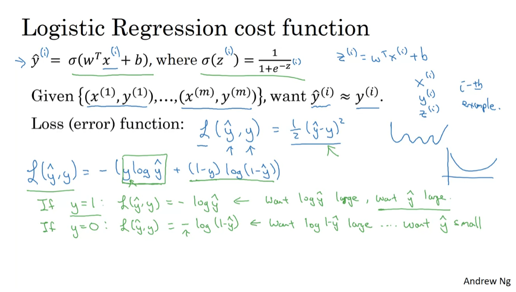
so what we use in logistic regression is
actually the following loss function, which I’m just going right
out here is negative. y log y hat plus 1 minus y log 1 minus, y hat here’s some intuition on why
this loss function makes sense. Keep in mind that if we’re using
squared error then you want to square error to be as small as possible. And with this logistic regression, lost function will also want
this to be as small as possible.

informal justification for this particular loss function

To understand why this makes sense,
let’s look at the two cases, in the first case let’s say y is
equal to 1, then the loss function. y hat comma Y is just this first
term right in this negative science, it’s negative log y
hat if y is equal to 1. Because if y equals 1, then the second
term 1 minus Y is equal to 0, so this says if y equals 1, you want negative
log y hat to be as small as possible. So that means you want log y hat to
be large to be as big as possible, and that means you want y hat to be large. But because y hat is you know the sigmoid
function, it can never be bigger than one. So this is saying that if y is equal to 1,
you want, y hat to be as big as possible,
but it can’t ever be bigger than one. So saying you want,
y hat to be close to one as well,

the other case is Y equals zero,
if Y equals 0. Then this first term in the loss function
is equal to 0 because y equals 0, and in the second term
defines the loss function. So the loss becomes negative
Log 1 minus y hat, and so if in your learning procedure you
try to make the loss function small. What this means is that you want,
Log 1 minus y hat to be large and
because it’s a negative sign there. And then through a similar piece of
reasoning, you can conclude that this loss function is trying to make
y hat as small as possible, and again, because y hat has
to be between zero and 1. This is saying that if y is equal to
zero then your loss function will push the parameters to make y
hat as close to zero as possible.

Now there are a lot of functions with
roughly this effect that if y is equal to one, try to make y hat large and
y is equal to zero or try to make y hat small. We just gave here in green a somewhat
informal justification for this particular loss function we will
provide an optional video later to give a more formal justification for y.

Cost function: which measures how are you doing on the entire training set

In logistic regression, we like to use the
loss function with this particular form. Finally, the last function was defined
with respect to a single training example. It measures how well you’re doing
on a single training example, I’m now going to define something
called the cost function, which measures how are you doing
on the entire training set. So the cost function j,
which is applied to your parameters W and B, is going to be the average,
really one of the m of the sun of the loss function apply to
each of the training examples. In turn, we’re here, y hat is of course
the prediction output by your logistic regression algorithm using, you know,
a particular set of parameters W and B. And so just to expand this out,
this is equal to negative one of them, some from I equals one through of
the definition of the lost function above. So this is y I log y hat I plus 1 minus Y, I log 1minus y hat I I guess it
can put square brackets here. So the minus sign is outside everything
else

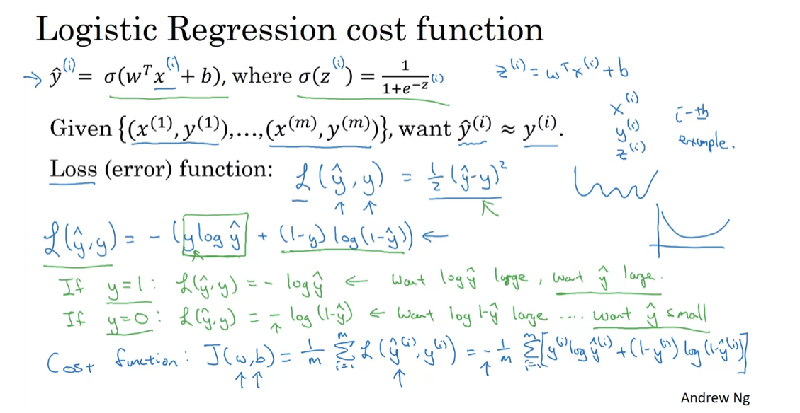
so the terminology I’m going to use is that the loss function is
applied to just a single training example. Like so and the cost function is the cost
of your parameters, so in training your logistic regression model, we’re
going to try to find parameters W and B. That minimize the overall cost function J,
written at the bottom.

So you’ve just seen the setup for
the logistic regression algorithm, the loss function for training example,
and the overall cost function for the parameters of your algorithm. It turns out that logistic
regression can be viewed as a very, very small neural network. In the next video, we’ll go over that so you can start gaining intuition
about what neural networks do. So with that let’s go on to the next video
about how to view logistic regression as a very small neural network.

Gradient Descent

You’ve seen the logistic regression model,
you’ve seen the loss function that measures how well you’re doing
on the single training example.

You’ve also seen the cost function that
measures how well your parameters W and B are doing on your entire training set.

gradient descent algorithm

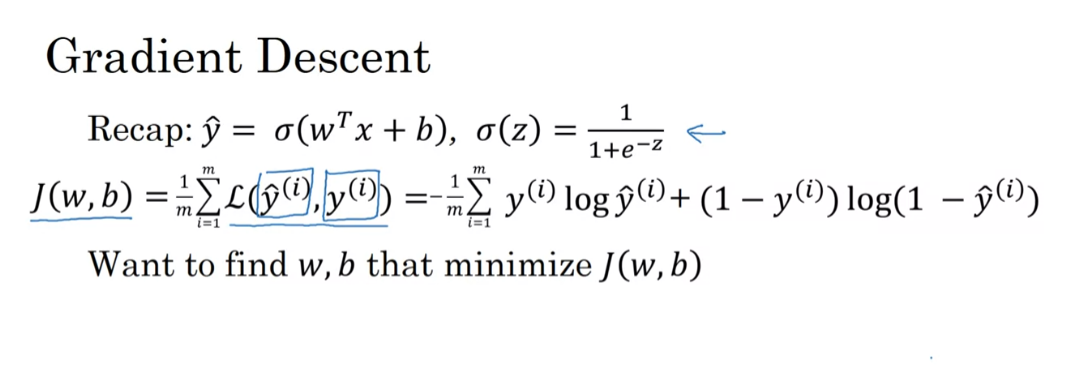
Now let’s talk about how you can use
the gradient descent algorithm to train or to learn the parameters
W on your training set.

To recap here is the familiar
logistic regression algorithm and we have on the second
line the cost function J, which is a function of
your parameters W and B.

And that’s defined as the average
is one over m times has some of this loss function.

And so the loss function measures
how well your algorithms outputs.

Y hat I on each of the training examples
stacks up compares to the boundary lables Y I on each of
the training examples.

The full formula is expanded out on the right.

So the cost function measures
how well your parameters w and b are doing on the training set.

So in order to learn a set
of parameters w and b, it seems natural that we
want to find w and b.

That make the cost function J of w,
b as small as possible.

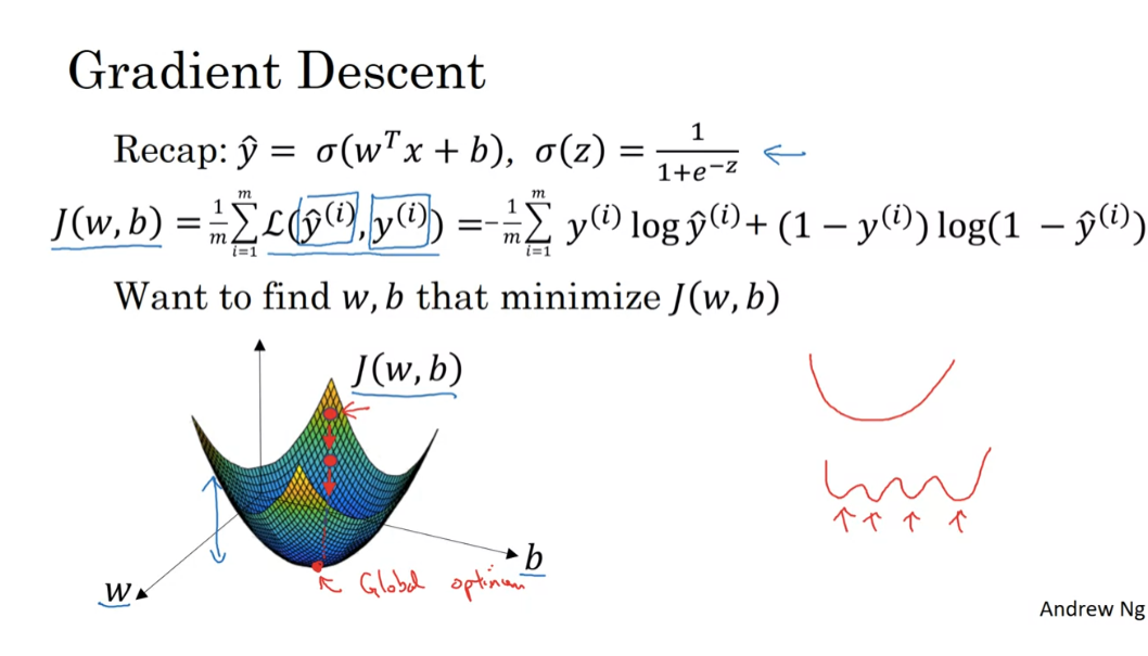
So, here’s an illustration
of gradient descent.

In this diagram, the horizontal axes
represent your space of parameters w and b in practice w can be much higher
dimensional, but for the purposes of plotting, let’s illustrate w as a singular number and b as a singular number.

The cost function J of w, b is then some surface above
these horizontal axes w and b.

The height of the surface represents the value of Cost function J

So the height of the surface represents
the value of J, b at a certain point.

And what we want to do really is
to find the value of w and b that corresponds to the minimum
of the cost function J.

It turns out that this particular
cost function J is a convex function.

A single big bowl, this is a convex function

So it’s just a single big bowl,
so this is a convex function and this is as opposed to
functions that look like this, which are non convex and
has lots of different local optimal.

So the fact that our cost function J of w, b as defined here is convex, is one of the huge reasons why we use this particular cost function J for logistic regression.

So the fact that our cost function J of w,
b as defined here is convex, is one of the huge reasons why we use
this particular cost function J for logistic regression.

So to find a good value for
the parameters, what we’ll do is initialize w and b to some initial value may be
denoted by that little red dot.

And for logistic regression,
almost any initialization method works.

Usually you Initialize the values of 0. Random initialization also works,
but people don’t usually do that for logistic regression.

But because this function is convex,
no matter where you initialize, you should get to the same point or
roughly the same point.

Start at an initial point and then takes a step in the steepest downhill direction.

And what gradient descent does is
it starts at that initial point and then takes a step in
the steepest downhill direction.

So after one step of gradient descent,
you might end up there because it’s trying to take a step downhill in
the direction of steepest descent or as quickly down who as possible.

So that’s one iteration
of gradient descent.

And after iterations of gradient descent, you might stop there, three iterations and
so on.

I guess this is not hidden by the back of
the plot until eventually, hopefully you converge to this global optimum or get to
something close to the global optimum.

So this picture illustrates
the gradient descent algorithm.

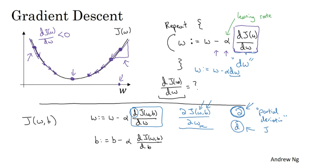
Let’s write a little bit more of the
details for the purpose of illustration, let’s say that there’s some function
J of w that you want to minimize and maybe that function looks like
this to make this easier to draw.

I’m going to ignore b for now just to make this one dimensional plot
instead of a higher dimensional plot.

So gradient descent does this. We’re going to repeatedly carry
out the following update.

We’ll take the value of w and update it. Going to use colon equals
to represent updating w.

So set w to w minus alpha times and this is a derivative d of J w d w.

And we repeatedly do that
until the algorithm converges.

So a couple of points in the notation
alpha here is the learning rate and controls how big a step we take on
each iteration are gradient descent, we’ll talk later about some ways for
choosing the learning rate, alpha and second this quantity here,
this is a derivative.

This is basically the update of the change
you want to make to the parameters w, when we start to write code to
implement gradient descent, we’re going to use the convention
that the variable name in our code, d w will be used to represent
this derivative term.

So when you write code,
you write something like w equals or cold equals w minus alpha time’s d w.

So we use d w to be the variable name
to represent this derivative term.

Just make sure that the gradient descent update makes sense.

Now, let’s just make sure that this
gradient descent update makes sense.

Let’s say that w was over here. So you’re at this point on
the cost function J of w.

Remember that the definition
of a derivative is the slope of a function at the point.

So the slope of the function is really, the height divided by the width
right of the lower triangle.

Here, in this tant to
J of w at that point.

And so here the derivative is positive.

W gets updated as w minus a learning
rate times the derivative, the derivative is positive.

And so you end up subtracting from w.

So you end up taking a step to the left
and so gradient descent with, make your algorithm slowly
decrease the parameter.

If you had started off with
this large value of w.

As another example, if w was over here, then at this point the slope here or
dJ detail, you will be negative.

And so they driven to send update with
subtract alpha times a negative number.

And so end up slowly increasing w.

So you end up you’re making w bigger and bigger with successive
generations of gradient descent.

So that hopefully whether you
initialize on the left, wonder right, create into central move you
towards this global minimum here.

If you’re not familiar with
derivatives of calculus and what this term d J of w d w means.

Don’t worry too much about it.

We’ll talk some more about
derivatives in the next video.

If you have a deep knowledge of calculus, you might be able to have a deeper
intuitions about how neural networks work.

But even if you’re not that familiar
with calculus in the next few videos will give you enough intuitions
about derivatives and about calculus that you’ll be able
to effectively use neural networks.

The overall intuition for now is that this term represents the slope of the function and we want to know the slope of the function at the current setting of the parameters so that we can take these steps of steepest descent so that we know what direction to step in in order to go downhill on the cost function J

But the overall intuition for now is that this term represents
the slope of the function and we want to know the slope of the function at
the current setting of the parameters so that we can take these steps of
steepest descent so that we know what direction to step in in order to go
downhill on the cost function J.

So we wrote our gradient descent for
J of w. If only w was your parameter
in logistic regression.

Your cost function is
a function above w and b.

In that case the inner
loop of gradient descent, that is this thing here the thing you
have to repeat becomes as follows.

You end up updating w as
w minus the learning rate times the derivative of
J of wb respect to w and you update b as b minus
the learning rate times the derivative of the cost
function respect to b.

So these two equations at the bottom of
the actual update you implement as in the side, I just want to mention one
notation, all convention and calculus.

That is a bit confusing to some people.

I don’t think it’s super important
that you understand calculus but in case you see this, I want to make sure
that you don’t think too much of this.

Which is that in calculus this term
here we actually write as follows, that funny squiggle symbol.

So this symbol,
this is actually just the lower case d in a fancy font,
in a stylized font.

But when you see this expression,
all this means is this is the of J of w, b or
really the slope of the function J of w, b how much that function
slopes in the w direction.

And the rule of the notation and calculus,
which I think is in total logical.

But the rule in the notation for
calculus, which I think just makes things much more complicated than you need to
be is that if J is a function of two or more variables,
then instead of using lower case d.

partial derivative symbol

You use this funny symbol. This is called a partial derivative
symbol, but don’t worry about this.

And if J is a function of only one
variable, then you use lower case d. So the only difference between whether you
use this funny partial derivative symbol or lower case d.

As we did on top is whether J is
a function of two or more variables.

In which case use this symbol,
the partial derivative symbol or J is only a function of one variable.

Then you use lower case d.

This is one of those funny
rules of notation and calculus that I think just make things
more complicated than they need to be.

But if you see this
partial derivative symbol, all it means is you’re measuring
the slope of the function with respect to one of the variables,
and similarly to adhere to the, formally correct mathematical notation
calculus because here J has two inputs. Not just one.

This thing on the bottom should be written
with this partial derivative simple, but it really means the same thing as,
almost the same thing as lowercase d.

Finally, when you implement this in code, we’re going to use the convention
that this quantity really the amount I wish you update w will denote
as the variable d w in your code.

And this quantity, right,
the amount by which you want to update b with the note by
the variable db in your code.

All right.

So that’s how you can
implement gradient descent.

Now if you haven’t seen calculus for a few
years, I know that that might seem like a lot more derivatives and calculus than
you might be comfortable with so far.

But if you’re feeling that way,
don’t worry about it.

In the next video will give you
better intuition about derivatives.

And even without the deep mathematical
understanding of calculus, with just an intuitive
understanding of calculus, you will be able to make your
networks work effectively so that let’s go into the next video, we’ll
talk a little bit more about derivatives.

Derivatives

Gain an intuitive understanding of calculus and the derivatives.

In this video, I want to help you gain an intuitive understanding, of calculus and the derivatives.

Now, maybe you’re thinking that you haven’t seen calculus since your college days, and depending on when you graduated, maybe that was quite some time back.

Now, if that’s what you’re thinking, don’t worry, you don’t need a deep understanding of calculus in order to apply neural networks and deep learning very effectively.

So, if you’re watching this video or some of the later videos and you’re wondering, well, is this stuff really for me, this calculus looks really complicated.

My advice to you is the following, which is that, watch the videos and then if you could do the homeworks and complete the programming homeworks successfully, then you can apply deep learning.

In fact, when you see later is that in week four, we’ll define a couple of types of functions that will enable you to encapsulate everything that needs to be done with respect to calculus, that these functions called forward functions and backward functions that you learn about.

That lets you put everything you need to know about calculus into these functions, so that you don’t need to worry about them anymore beyond that.

But I thought that in this foray into deep learning that this week, we should open up the box and peer a little bit further into the details of calculus.

But really, all you need is an intuitive understanding of this in order to build and successfully apply these algorithms.

Finally, if you are among that maybe smaller group of people that are expert in calculus, if you are very familiar with calculus derivatives, it’s probably okay for you to skip this video.

But for everyone else, let’s dive in, and try to gain an intuitive understanding of derivatives.

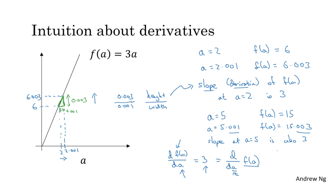
I plotted here the function f(a) equals 3a.

So, it’s just a straight line.

To get intuition about derivatives, let’s look at a few points on this function.

Let say that a is equal to two.

In that case, f of a, which is equal to three times a is equal to six. So, if a is equal to two, then f of a will be equal to six.

Let’s say we give the value of a just a little bit of a nudge.

I’m going to just bump up a, a little bit, so that it is now 2.001. So, I’m going to give a like a tiny little nudge, to the right. So now, let’s say 2.001, just plot this into scale, 2.001, this 0.001 difference is too small to show on this plot, just give a little nudge to that right.

Now, f(a), is equal to three times that. So, it’s 6.003, so we plot this over here.

This is not to scale, this is 6.003.

So, if you look at this little triangle here that I’m highlighting in green, what we see is that if I nudge a 0.001 to the right, then f of a goes up by 0.003.

The amounts that f of a, went up is three times as big as the amount that I nudge the a to the right.

So, we’re going to say that, the slope or the derivative of the function f of a, at a equals to or when a is equals two to the slope is three.

The term derivative basically means slope, it’s just that derivative sounds like a scary and more intimidating word, whereas a slope is a friendlier way to describe the concept of derivative.

The term derivative basically means slope, it’s just that derivative sounds like a scary and more intimidating word, whereas a slope is a friendlier way to describe the concept of derivative.

So, whenever you hear derivative, just think slope of the function.

More formally, the slope is defined as the height divided by the width of this little triangle that we have in green.

So, this is 0.003 over 0.001, and the fact that the slope is equal to three or the derivative is equal to three, just represents the fact that when you nudge a to the right by 0.001, by tiny amount, the amount at f of a goes up is three times as big as the amount that you nudged it, that you nudged a in the horizontal direction.

So, that’s all that the slope of a line is.

Now, let’s look at this function at a different point.

Let’s say that a is now equal to five. In that case, f of a, three times a is equal to 15. So, let’s see that again, give a, a nudge to the right.

A tiny little nudge, it’s now bumped up to 5.001, f of a is three times that. So, f of a is equal to 15.003. So, once again, when I bump a to the right, nudge a to the right by 0.001, f of a goes up three times as much. So the slope, again, at a = 5, is also three.

So, the way we write this, that the slope of the function f is equal to three: We say, d f(a) da and this just means, the slope of the function f(a) when you nudge the variable a, a tiny little amount, this is equal to three.

But all this equation means is that, if I nudge a to the right a little bit, I expect f(a) to go up by three times as much as I nudged the value of little a.

An alternative way to write this derivative formula is as follows.

You can also write this as, d da of f(a). So, whether you put f(a) on top or whether you write it down here, it doesn’t matter.

But all this equation means is that, if I nudge a to the right a little bit, I expect f(a) to go up by three times as much as I nudged the value of little a.

Now, for this video I explained derivatives, talking about what happens if we nudged the variable a by 0.001.

If you want a formal mathematical definition of the derivatives: Derivatives are defined with an even smaller value of how much you nudge a to the right. So, it’s not 0.001. It’s not 0.000001. It’s not 0.00000000 and so on 1.

It’s even smaller than that, and the formal definition of derivative says, whenever you nudge a to the right by an infinitesimal amount, basically an infinitely tiny, tiny amount.

If you do that, this f(a) go up three times as much as whatever was the tiny, tiny, tiny amount that you nudged a to the right.

So, that’s actually the formal definition of a derivative.

But for the purposes of our intuitive understanding, which I’ll talk about nudging a to the right by this small amount 0.001.

Even if it’s 0.001 isn’t exactly tiny, tiny infinitesimal.

Now, one property of the derivative is that, no matter where you take the slope of this function, it is equal to three, whether a is equal to two or a is equal to five.

The slope of this function is equal to three, meaning that whatever is the value of a, if you increase it by 0.001, the value of f of a goes up by three times as much.

So, this function has a safe slope everywhere.

One way to see that is that, wherever you draw this little triangle. The height, divided by the width, always has a ratio of three to one.

So, I hope this gives you a sense of what the slope or the derivative of a function means for a straight line, where in this example the slope of the function was three everywhere.

In the next video, let’s take a look at a slightly more complex example, where the slope to the function can be different at different points on the function.

More Derivative Examples

The slope of the function can be different to different points in the function.

In this video, I’ll show you a
slightly more complex example where the slope of the function can be
different to different points in the function.

Let’s start with an example.

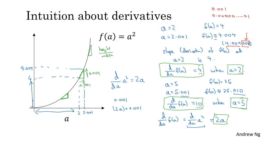
You have plotted the function f(a) = a². Let’s take a look at the point a=2. So a² or f(a) = 4.

Let’s nudge a slightly to
the right, so now a=2.001. f(a) which is a² is going to
be approximately 4.004.

It turns out that the exact value, you call the calculator and figured
this out is actually 4.004001. I’m just going to say
4.004 is close enough.

So what this means is that when a=2, let’s draw this on the plot. So what we’re saying is that if a=2, then f(a) = 4 and here is the
x and y axis are not drawn to scale.

Technically, does vertical height
should be much higher than this horizontal height so the
x and y axis are not on the same scale.

But if I now nudge a to 2.001
then f(a) becomes roughly 4.004. So if we draw this little triangle again, what this means is that if
I nudge a to the right by 0.001, f(a) goes up four times as much by 0.004. So in the language of calculus, we say that a slope that is
the derivative of f(a) at a=2 is 4 or to write this out
of our calculus notation, we say that d/da of f(a) = 4 when a=2.

Now one thing about this function f(a) = a² is that the slope is different
for different values of a.

This is different than the example
we saw on the previous slide.

So let’s look at a different point. If a=5, so instead of a=2, and now a=5 then a²=25, so that’s f(a). If I nudge a to the right again, it’s tiny little nudge to a, so now a=5.001 then f(a) will be
approximately 25.010.

So what we see is that by
nudging a up by .001, f(a) goes up ten times as much. So we have that d/da f(a) = 10 when a=5 because f(a) goes up ten times as much as a does when I make a
tiny little nudge to a.

So one way to see why did derivatives is
different at different points is that if you draw that little triangle right at
different locations on this, you’ll see that the ratio of the
height of the triangle over the width of the triangle is very
different at different points on the curve.

So here, the slope=4
when a=2, a=10, when a=5. Now if you pull up a calculus textbook, a calculus textbook will
tell you that d/da of f(a), so f(a) = a², so that’s d/da of a².

One of the formulas you find are
the calculus textbook is that this thing, the slope of the function a²,
is equal to 2a. Not going to prove this, but
the way you find this out is that you open up a calculus textbook to the table formulas and they’ll tell you
that derivative of 2 of a² is 2a.

And indeed, this is consistent with
what we’ve worked out. Namely, when a=2, the slope of
function to a is 2x2=4. And when a=5 then the slope of
the function 2xa is 2x5=10.

So, if you ever pull up a calculus
textbook and you see this formula, that the derivative of a²=2a, all that means is that for
any given value of a, if you nudge upward by 0.001
already your tiny little value, you will expect f(a) to go up by 2a. That is the slope or the derivative times other much you had nudged
to the right the value of a.

Now one tiny little detail, I use these approximate symbols here
and this wasn’t exactly 4.004, there’s an extra .001 hanging out there. It turns out that this extra .001, this little thing here is because
we were nudging a to the right by 0.001, if we’re instead nudging it
to the right by this infinitesimally small value
then this extra every term will go away and you find that the amount that
f(a) goes out is exactly equal to the derivative times the amount
that you nudge a to the right. And the reason why is not 4.004 exactly is
because derivatives are defined using this infinitesimally small nudges to a
rather than 0.001 which is not.

And while 0.001 is small, it’s not infinitesimally small. So that’s why the amount that
f(a) went up isn’t exactly given by the formula but it’s only a kind of
approximately given by the derivative.

To wrap up this video, let’s just go through a
few more quick examples.

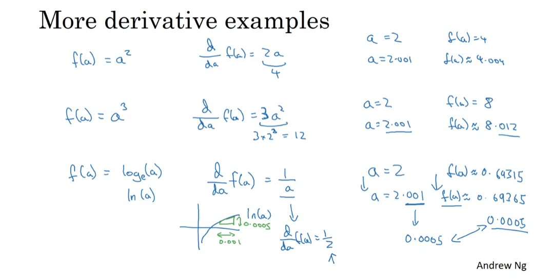
The example you’ve already seen
is that if f(a) = a² then the calculus textbooks formula table will
tell you that the derivative is equal to 2a.

And so the example we went through
was it if (a) = 2, f(a) = 4, and we nudge a, since it’s a little bit
bigger than f(a) is about 4.004 and so f(a) went up four times
as much and indeed when a=2, the derivatives is equal to 4.

Let’s look at some other examples. Let’s say, instead the f(a) = a³. If you go to a calculus textbook
and look up the table of formulas, you see that the slope of
this function, again, the derivative of this function
is equal to 3a².

So you can get this formula
out of the calculus textbook.

So what this means? So the way to interpret
this is as follows.

Let’s take a=2 as an example again.

So f(a) or a³=8, that’s
two to the power of three.

So we give a a tiny little nudge, you find that f(a) is about 8.012
and feel free to check this. Take 2.001 to the power of three, you find this is very close to 8.012.

And indeed, when a=2 that’s
3x2² does equal to 3x4, you see that’s 12. So the derivative formula predicts that if
you nudge a to the right by tiny little bit, f(a) should go up 12 times as much.

And indeed, this is true
when a went up by .001, f(a) went up 12 times as much by .012. Just one last example
and then we’ll wrap up.

Let’s say that f(a) is equal to
the log function. So on the right log of a, I’m going to use this as
the base e logarithm.

So some people write that as log(a).

So if you go to calculus textbook, you find that when you take the
derivative of log(a).

So this is a function that
just looks like that, the slope of this function is
given by 1/a. So the way to interpret this is that
if a has any value then let’s just keep using a=2 as an example and you
nudge a to the right by .001, you would expect f(a) to go up by 1/a that is by the derivative times
the amount that you increase a.

So in fact, if you pull up a calculator, you find that if a=2, f(a) is about 0.69315 and if you increase f and if you increase a to
2.001 then f(a) is about 0.69365, this has gone up by 0.0005.

And indeed, if you look at the formula
for the derivative when a=2, d/da f(a) = 1/2.

So this derivative formula predicts
that if you pump up a by .001, you would expect f(a) to go up by
only 1/2 as much and 1/2 of .001 is 0.0005 which is exactly what we got.

Then when a goes up by .001,
going from a=2 to a=2.001, f(a) goes up by half as much. So, the answers are going up by
approximately .0005.

So if we draw that little triangle
if you will is that if on the horizontal axis just goes up by
.001 on the vertical axis, log(a) goes up by half of that so .0005.

And so that 1/a or 1/2 in this case, 1a=2 that’s just the slope of
this line when a=2.

So that’s it for derivatives.

Two take home messages

First is that the derivative of the function just means the slope of a function and the slope of a function can be different at different points on the function.

There are just two take home messages
from this video.

First is that the derivative of the
function just means the slope of a function and the slope of a function can be different at different
points on the function.

In our first example where
f(a) = 3a those a straight line.

The derivative was the same everywhere, it was three everywhere.

For other functions like
f(a) = a² or f(a) = log(a), the slope of the line varies.

So, the slope or the derivative can be
different at different points on the curve.

So that’s a first take away. Derivative just means slope of a line.

The second takeaway

Second takeaway is that if you want to
look up the derivative of a function, you can flip open your calculus textbook
or look up Wikipedia and often get a formula for the slope of
these functions at different points.

So that, I hope you have an intuitive
understanding of derivatives or slopes of lines. Let’s go into the next video. We’ll start to talk about the
computation graph and how to use that to compute derivatives of
more complex functions.

Computation Graph

You’ve heard me say that the computations of a neural network are organized in terms of a forward pass or a forward propagation step, in which we compute the output of the neural network, followed by a backward pass or back propagation step, which we use to compute gradients or compute derivatives.

The computation graph explains why it is organized this way.

In this video, we’ll go through an example.

In order to illustrate the computation graph, let’s use a simpler example than logistic regression or a full blown neural network.

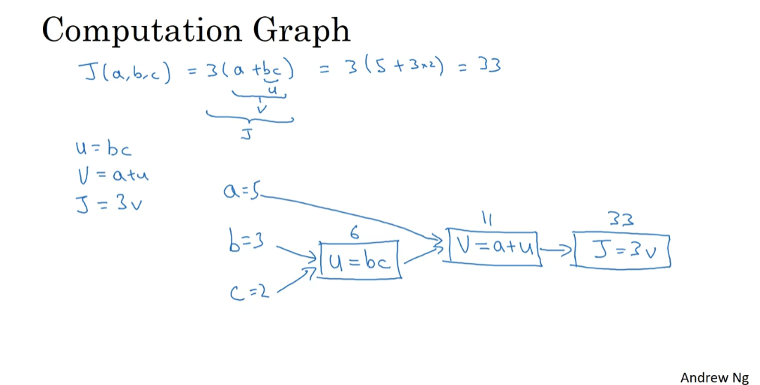
Let’s say that we’re trying to compute a function, J, which is a function of three variables a, b, and c and let’s say that function is 3(a+bc).

Has three distinct steps

Computing this function actually has three distinct steps.

The first is you need to compute what is bc and let’s say we store that in the variable call u.

So u=bc and then you my compute V=a *u. So let’s say this is V.

And then finally, your output J is 3V.

So this is your final function J that you’re trying to compute.

Draw the computation steps in a computation graph

We can take these three steps and draw them in a computation graph as follows.

Let’s say, I draw your three variables a, b, and c here.

So the first thing we did was compute u=bc.

So I’m going to put a rectangular box around that.

And so the input to that are b and c.

And then, you might have V=a+u.

So the inputs to that are V. So the inputs to that are u with just computed together with a.

And then finally, we have J=3V.

So as a concrete example, if a=5, b=3 and c=2 then u=bc would be six because a+u would be 5+6 is 11,. J is three times that, so J=33.

And indeed, hopefully you can verify that this is three times five plus three times two.

And if you expand that out, you actually get 33 as the value of J.

So, the computation graph comes in handy when there is some distinguished or some special output variable, such as J in this case, that you want to optimize.

And in the case of a logistic regression, J is of course the cost function that we’re trying to minimize.

And what we’re seeing in this little example is that, through a left-to-right pass, you can compute the value of J and what we’ll see in the next couple of slides is that in order to compute derivatives there’ll be a right-to-left pass like this, kind of going in the opposite direction as the blue arrows.

That would be most natural for computing the derivatives.

So to recap, the computation graph organizes a computation with this blue arrow, left-to-right computation. Let’s refer to the next video how you can do the backward red arrow right-to-left computation of the derivatives. Let’s go on to the next video.

Derivatives with a Computation Graph

In the last video, we worked through an example of using a
computation graph to compute a function J. Now, let’s take a cleaned up version
of that computation graph and show how you can use it to figure
out derivative calculations for that function J.

So here’s a computation graph. Let’s say you want to compute
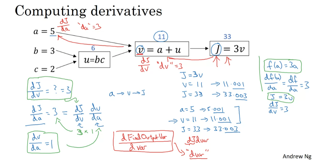
the derivative of J with respect to v. So what is that? Well, this says,
if we were to take this value of v and change it a little bit,
how would the value of J change? Well, J is defined as 3 times v. And right now, v = 11. So if we’re to bump up v
by a little bit to 11.001, then J, which is 3v, so currently 33, will get bumped up to 33.003. So here, we’ve increased v by 0.001. And the net result of that is
that J goes up 3 times as much. So the derivative of J with
respect to v is equal to 3. Because the increase in J is
3 times the increase in v.

And in fact,
this is very analogous to the example we had in the previous video,
where we had f(a) = 3a. And so we then derived that df/da,
which with slightly simplified, a slightly sloppy notation,
you can write as df/da = 3. So instead, here we have J = 3v, and so dJ/dv = 3.

With here, J playing the role of f, and v playing the role of a in this previous
example that we had from an earlier video. So indeed, terminology of backpropagation,
what we’re seeing is that if you want to compute the
derivative of this final output variable, which usually is a variable
you care most about, with respect to v, then we’ve
done one step of backpropagation. So we call it one step
backwards in this graph.

Now let’s look at another example. What is dJ/da? In other words, if we bump up the value of
a, how does that affect the value of J? Well, let’s go through the example,
where now a = 5. So let’s bump it up to 5.001. The net impact of that is that v, which
was a + u, so that was previously 11. This would get increased to 11.001. And then we’ve already seen as above that J now gets bumped up to 33.003.

So what we’re seeing is that if you
increase a by 0.001, J increases by 0.003. And by increase a, I mean,
you have to take this value of 5 and just plug in a new value. Then the change to a will propagate to
the right of the computation graph so that J ends up being 33.003. And so the increase to J is
3 times the increase to a. So that means this
derivative is equal to 3.

And one way to break this down
is to say that if you change a, then that will change v. And through changing v,
that would change J. And so the net change to the value
of J when you bump up the value, when you nudge the value of
a up a little bit, is that, First, by changing a,
you end up increasing v. Well, how much does v increase? It is increased by an amount
that’s determined by dv/da. And then the change in v will cause
the value of J to also increase.

So in calculus, this is actually called
the chain rule that if a affects v, affects J,
then the amounts that J changes when you nudge a is the product of
how much v changes when you nudge a times how much J
changes when you nudge v. So in calculus, again,
this is called the chain rule.

And what we saw from this calculation
is that if you increase a by 0.001, v changes by the same amount. So dv/da = 1. So in fact, if you plug in what
we have wrapped up previously, dv/dJ = 3 and dv/da = 1. So the product of these 3 times 1, that actually gives you
the correct value that dJ/da = 3. So this little illustration shows
hows by having computed dJ/dv, that is,
derivative with respect to this variable, it can then help you to compute dJ/da. And so that’s another step of
this backward calculation.

I just want to introduce one
more new notational convention. Which is that when you’re witting
codes to implement backpropagation, there will usually be some final output
variable that you really care about. So a final output variable that you really
care about or that you want to optimize. And in this case,
this final output variable is J. It’s really the last node
in your computation graph. And so a lot of computations will be
trying to compute the derivative of that final output variable. So d of this final output variable
with respect to some other variable. Then we just call that dvar.

So a lot of the computations you have will
be to compute the derivative of the final output variable, J in this case,
with various intermediate variables, such as a, b, c, u or v. And when you implement this in software,
what do you call this variable name? One thing you could do is in Python, you could give us a very long variable
name like dFinalOurputVar/dvar. But that’s a very long variable name. You could call this, I guess, dJdvar. But because you’re always taking
derivatives with respect to dJ, with respect to this final output variable,
I’m going to introduce a new notation. Where, in code, when you’re computing
this thing in the code you write, we’re just going to use the variable name
dvar in order to represent that quantity. So dvar in a code you write will
represent the derivative of the final output variable
you care about such as J.

Well, sometimes, the last l with respect
to the various intermediate quantities you’re computing in your code. So this thing here in your code,
you use dv to denote this value. So dv would be equal to 3. And your code, you represent this as da, which is we also figured
out to be equal to 3.

So we’ve done backpropagation partially
through this computation graph. Let’s go through the rest of
this example on the next slide. So let’s go to a cleaned up
copy of the computation graph. And just to recap, what we’ve done so far is go backward here and
figured out that dv = 3. And again, the definition of dv,
that’s just a variable name, where the code is really dJ/dv. We’ve figured out that da = 3. And again, da is the variable name in your
code and that’s really the value dJ/da.

And we hand wave how we’ve gone
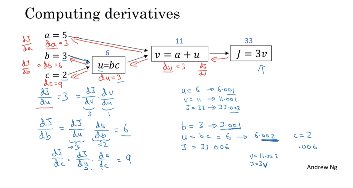
backwards on these two edges like so. Now let’s keep computing derivatives. Now let’s look at the value u. So what is dJ/du? Well, through a similar calculation
as what we did before and then we start off with u = 6. If you bump up u to 6.001, then v, which is previously 11, goes up to 11.001. And so J goes from 33 to 33.003. And so the increase in J is 3x,
so this is equal. And the analysis for u is very
similar to the analysis we did for a. This is actually computed
as dJ/dv times dv/du, where this we had already
figured out was 3. And this turns out to be equal to 1.

So we’ve gone up one more
step of backpropagation. We end up computing that
du is also equal to 3. And du is, of course, just this dJ/du. Now we just step through
one last example in detail. So what is dJ/db?

So here, imagine if you are allowed
to change the value of b. And you want to tweak b a little
bit in order to minimize or maximize the value of J. So what is the derivative or what’s the slope of this function J when
you change the value of b a little bit? It turns out that using the chain rule for
calculus, this can be written as
the product of two things. This dJ/du times du/db. And the reasoning is if
you change b a little bit, so b = 3 to, say, 3.001. The way that it will affect
J is it will first affect u. So how much does it affect u? Well, u is defined as b times c. So this will go from 6, when b = 3, to now 6.002 because c = 2 in our example here.

And so this tells us that du/db = 2. Because when you bump up b by 0.001,
u increases twice as much. So du/db, this is equal to 2. And now, we know that u has gone
up twice as much as b has gone up. Well, what is dJ/du? We’ve already figured out
that this is equal to 3. And so by multiplying these two out,
we find that dJ/db = 6. And again, here’s the reasoning for
the second part of the argument. Which is we want to know when u goes
up by 0.002, how does that affect J? The fact that dJ/du = 3,
that tells us that when u goes up by 0.002,
J goes up 3 times as much. So J should go up by 0.006. So this comes from
the fact that dJ/du = 3.

And if you check the math in detail, you will find that if b becomes 3.001, then u becomes 6.002, v becomes 11.002. So that’s a + u, so that’s 5 + u. And then J, which is equal to 3 times v, that ends up being equal to 33.006. And so that’s how you get that dJ/db = 6. And to fill that in, this is if we
go backwards, so this is db = 6. And db really is the Python
code variable name for dJ/db.

And I won’t go through the last
example in great detail. But it turns out that if
you also compute out dJ, this turns out to be dJ/du times du. And this turns out to be 9,
this turns out to be 3 times 3. I won’t go through that example in detail. So through this last step, it is
possible to derive that dc is equal to 9.

So the key takeaway from this video,
from this example, is that when computing derivatives and computing all of these
derivatives, the most efficient way to do so is through a right to left computation
following the direction of the red arrows. And in particular, we’ll first compute
the derivative with respect to v. And then that becomes useful for computing the derivative with respect to
a and the derivative with respect to u. And then the derivative with respect to u,
for example, this term over here and
this term over here. Those in turn become useful for computing
the derivative with respect to b and the derivative with respect to c.

So that was the computation graph and
how does a forward or left to right calculation to compute the cost function
such as J that you might want to optimize. And a backwards or a right to left
calculation to compute derivatives. If you’re not familiar with calculus or
the chain rule, I know some of those details, but
they’ve gone by really quickly. But if you didn’t follow all the details,
don’t worry about it. In the next video, we’ll go over this again in
the context of logistic regression. And show you exactly what you need to do
in order to implement the computations you need to compute the derivatives
of the logistic regression model.

Logistic Regression Gradient Descent

Welcome back. In this video, we’ll talk about how to compute derivatives for you to implement gradient descent for logistic regression. The key takeaways will be what you need to implement. That is, the key equations you need in order to implement gradient descent for logistic regression. In this video, I want to do this computation using the computation graph. I have to admit, using the computation graph is a little bit of an overkill for deriving gradient descent for logistic regression, but I want to start explaining things this way to get you familiar with these ideas so that, hopefully, it will make a bit more sense when we talk about full-fledged neural networks.

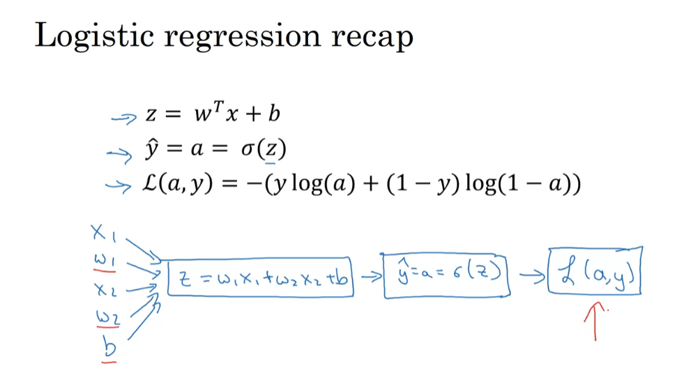
To that, let’s dive into gradient descent for logistic regression. To recap, we had set up logistic regression as follows, your predictions, Y_hat, is defined as follows, where z is that. If we focus on just one example for now, then the loss, or respect to that one example, is defined as follows, where A is the output of logistic regression, and Y is the ground truth label.

Let’s write this out as a computation graph and for this example, let’s say we have only two features, X1 and X2. In order to compute Z, we’ll need to input W1, W2, and B, in addition to the feature values X1, X2. These things, in a computational graph, get used to compute Z, which is W1, X1 + W2 X2 + B, rectangular box around that.

Then, we compute Y_hat, or A = Sigma_of_Z, that’s the next step in the computation graph, and then, finally, we compute L, AY, and I won’t copy the formula again.

In logistic regression, what we want to do is to modify the parameters, W and B, in order to reduce this loss. We’ve described the forward propagation steps of how you actually compute the loss on a single training example, now let’s talk about how you can go backwards to compute the derivatives.

Here’s a cleaned-up version of the diagram. Because what we want to do is compute derivatives with respect to this loss, the first thing we want to do when going backwards is to compute the derivative of this loss with respect to, the script over there, with respect to this variable A. So, in the code, you just use DA to denote this variable.

It turns out that if you are familiar with calculus, you could show that this ends up being -Y_over_A+1-Y_over_1-A. And the way you do that is you take the formula for the loss and, if you’re familiar with calculus, you can compute the derivative with respect to the variable, lowercase A, and you get this formula. But if you’re not familiar with calculus, don’t worry about it. We’ll provide the derivative formulas, what else you need, throughout this course.

If you are an expert in calculus, I encourage you to look up the formula for the loss from their previous slide and try taking derivative with respect to A using calculus, but if you don’t know enough calculus to do that, don’t worry about it. Now, having computed this quantity of DA and the derivative or your final alpha variable with respect to A, you can then go backwards.

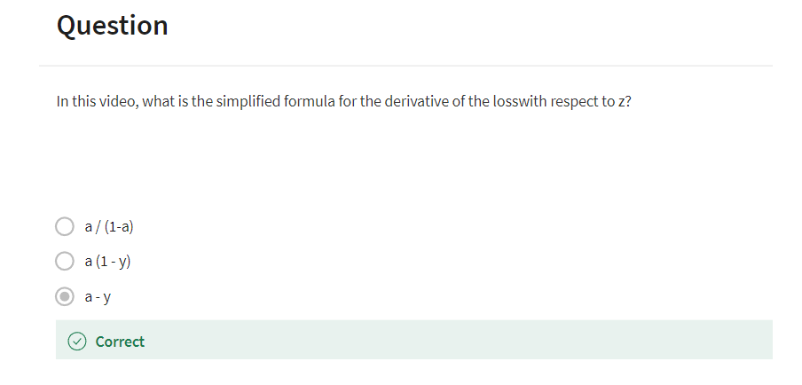
It turns out that you can show DZ which, this is the part called variable name, this is going to be the derivative of the loss, with respect to Z, or for L, you could really write the loss including A and Y explicitly as parameters or not, right? Either type of notation is equally acceptable. We can show that this is equal to A-Y. Just a couple of comments only for those of you experts in calculus, if you’re not expert in calculus, don’t worry about it. But it turns out that this, DL DZ, this can be expressed as DL_DA_times_DA_DZ, and it turns out that DA DZ, this turns out to be A_times_1-A, and DL DA we have previously worked out over here, if you take these two quantities, DL DA, which is this term, together with DA DZ, which is this term, and just take these two things and multiply them. You can show that the equation simplifies to A-Y.

That’s how you derive it, and that this is really the chain rule that have briefly eluded to the form. Feel free to go through that calculation yourself if you are knowledgeable in calculus, but if you aren’t, all you need to know is that you can compute DZ as A-Y and we’ve already done that calculus for you.

Then, the final step in that computation is to go back to compute how much you need to change W and B. In particular, you can show that the derivative with respect to W1 and in quotes, call this DW1, that this is equal to X1_times_DZ. Then, similarly, DW2, which is how much you want to change W2, is X2_times_DZ and B, excuse me, DB is equal to DZ.

If you want to do gradient descent with respect to just this one example, what you would do is the following; you would use this formula to compute DZ, and then use these formulas to compute DW1, DW2, and DB, and then you perform these updates. W1 gets updated as W1 minus, learning rate alpha, times DW1. W2 gets updated similarly, and B gets set as B minus the learning rate times DB. And so, this will be one step of grade with respect to a single example.

You see in how to compute derivatives and implement gradient descent for logistic regression with respect to a single training example. But training logistic regression model, you have not just one training example given training sets of M training examples. In the next video, let’s see how you can take these ideas and apply them to learning, not just from one example, but from an entire training set.

Gradient Descent on m Examples

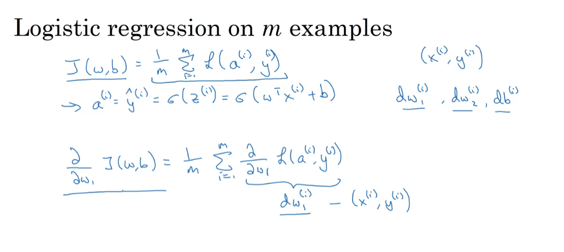
In a previous video, you saw how to compute derivatives and implement gradient descent with respect to just one training example for logistic regression. Now, we want to do it for m training examples. To get started, let’s remind ourselves of the definition of the cost function J. Cost- function w,b,which you care about is this average, one over m sum from i equals one through m of the loss when you algorithm output a_i on the example y, where a_i is the prediction on the ith training example which is sigma of z_i, which is equal to sigma of w transpose x_i plus b.

So, what we show in the previous slide is for any single training example, how to compute the derivatives when you have just one training example. So dw_1, dw_2 and d_b, with now the superscript i to denote the corresponding values you get if you were doing what we did on the previous slide, but just using the one training example, x_i y_i, excuse me, missing an i there as well.

So, now you notice the overall cost functions as a sum was really average, because the one over m term of the individual losses. So, it turns out that the derivative, respect to w_1 of the overall cost function is also going to be the average of derivatives respect to w_1 of the individual loss terms. But previously, we have already shown how to compute this term as dw_1_i, which we, on the previous slide, show how to compute this on a single training example.

So, what you need to do is really compute these derivatives as we showed on the previous training example and average them, and this will give you the overall gradient that you can use to implement the gradient descent.

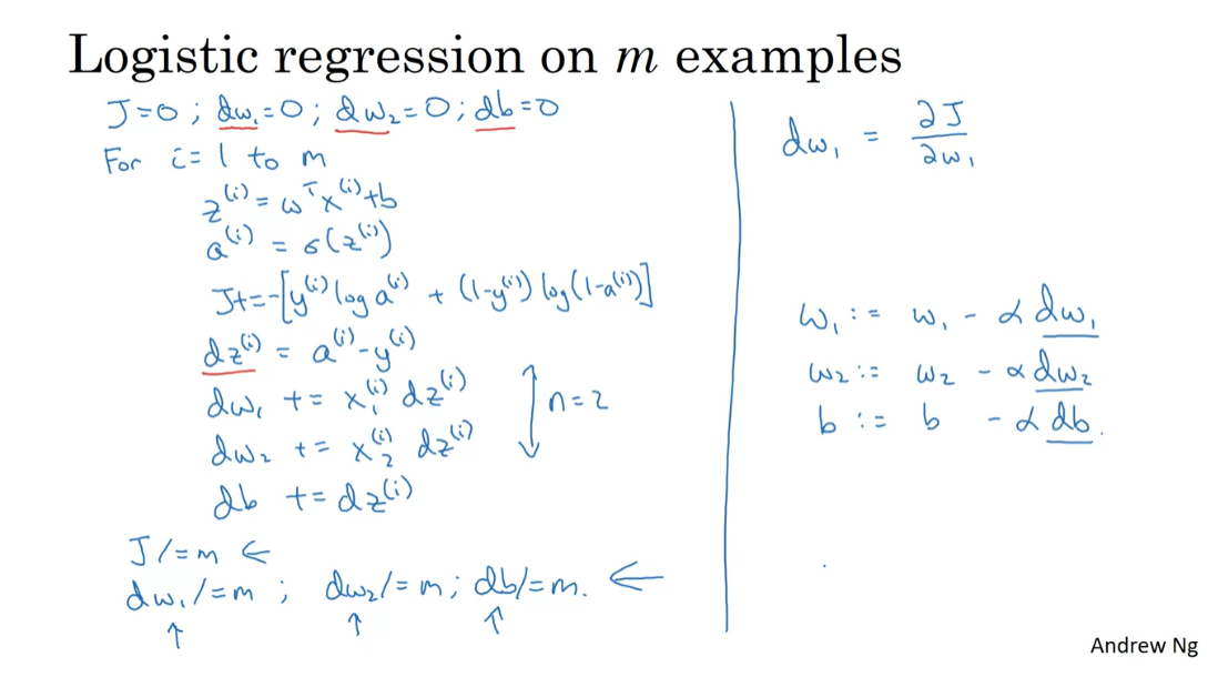
So, I know that was a lot of details, but let’s take all of this up and wrap this up into a concrete algorithm until when you should implement logistic regression with gradient descent working. So, here’s what you can do: let’s initialize j equals zero, dw_1 equals zero, dw_2 equals zero, d_b equals zero. What we’re going to do is use a for loop over the training set, and compute the derivative with respect to each training example and then add them up.

So, here’s how we do it, for i equals one through m, so m is the number of training examples, we compute z_i equals w transpose x_i plus b. The prediction a_i is equal to sigma of z_i, and then let’s add up J, J plus equals y_i log a_i plus one minus y_i log one minus a_i, and then put the negative sign in front of the whole thing, and then as we saw earlier, we have dz_i, that’s equal to a_i minus y_i, and d_w gets plus equals x1_i dz_i, dw_2 plus equals xi_2 dz_i, and I’m doing this calculation assuming that you have just two features, so that n equals to two otherwise, you do this for dw_1, dw_2, dw_3 and so on, and then db plus equals dz_i, and I guess that’s the end of the for loop.

Then finally, having done this for all m training examples, you will still need to divide by m because we’re computing averages. So, dw_1 divide equals m, dw_2 divides equals m, db divide equals m, in order to compute averages. So, with all of these calculations, you’ve just computed the derivatives of the cost function J with respect to each your parameters w_1, w_2 and b.

Just a couple of details about what we’re doing, we’re using dw_1 and dw_2 and db as accumulators, so that after this computation, dw_1 is equal to the derivative of your overall cost function with respect to w_1 and similarly for dw_2 and db. So, notice that dw_1 and dw_2 do not have a superscript i, because we’re using them in this code as accumulators to sum over the entire training set. Whereas in contrast, dz_i here, this was dz with respect to just one single training example. So, that’s why that had a superscript i to refer to the one training example, i that is computerised.

So, having finished all these calculations, to implement one step of gradient descent, you will implement w_1, gets updated as w_1 minus the learning rate times dw_1, w_2, ends up this as w_2 minus learning rate times dw_2, and b gets updated as b minus the learning rate times db, where dw_1, dw_2 and db were as computed.

Finally, J here will also be a correct value for your cost function. So, everything on the slide implements just one single step of gradient descent, and so you have to repeat everything on this slide multiple times in order to take multiple steps of gradient descent.

In case these details seem too complicated, again, don’t worry too much about it for now, hopefully all this will be clearer when you go and implement this in the programming assignments.

But it turns out there are two weaknesses with the calculation as we’ve implemented it here, which is that, to implement logistic regression this way, you need to write two for loops. The first for loop is this for loop over the m training examples, and the second for loop is a for loop over all the features over here. So, in this example, we just had two features; so, n is equal to two and x equals two, but maybe we have more features, you end up writing here dw_1 dw_2, and you similar computations for dw_t, and so on delta dw_n. So, it seems like you need to have a for loop over the features, over n features.

When you’re implementing deep learning algorithms, you find that having explicit for loops in your code makes your algorithm run less efficiency. So, in the deep learning era, we would move to a bigger and bigger datasets, and so being able to implement your algorithms without using explicit for loops is really important and will help you to scale to much bigger datasets.

So, it turns out that there are a set of techniques called vectorization techniques that allow you to get rid of these explicit for-loops in your code. I think in the pre-deep learning era, that’s before the rise of deep learning, vectorization was a nice to have, so you could sometimes do it to speed up your code and sometimes not. But in the deep learning era, vectorization, that is getting rid of for loops, like this and like this, has become really important, because we’re more and more training on very large datasets, and so you really need your code to be very efficient.

So, in the next few videos, we’ll talk about vectorization and how to implement all this without using even a single for loop. So, with this, I hope you have a sense of how to implement logistic regression or gradient descent for logistic regression. Things will be clearer when you implement the programming exercise. But before actually doing the programming exercise, let’s first talk about vectorization so that you can implement this whole thing, implement a single iteration of gradient descent without using any for loops.

Derivation of DL/dz (Optional)

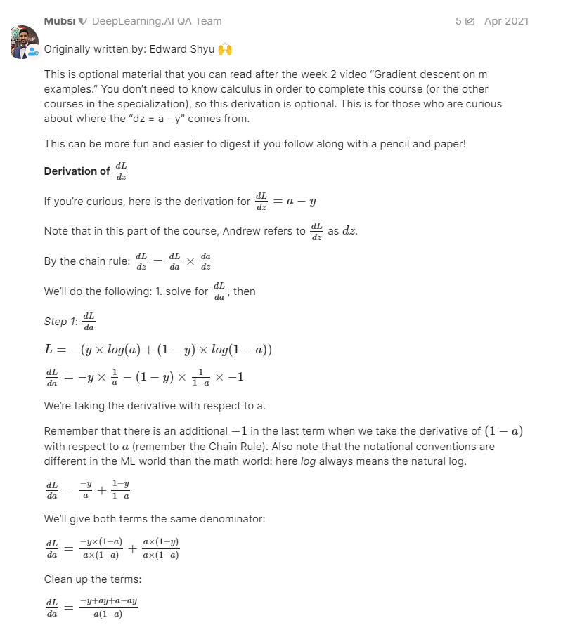
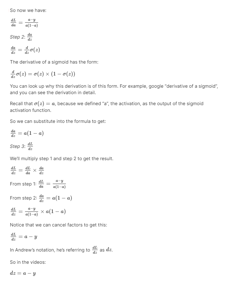
Derivation of $\frac{dL}{dz}$

If you’re curious, you can find the derivation for $\frac{dL}{dz}=a-y$ in this Discourse post “Derivation of DL/dz”

Remember that you do not need to know calculus in order to complete this course or the other courses in this specialization. The derivation is just for those who are curious about how this is derived.

[2] Python and Vectorization

Vectorization

Welcome back. Vectorization is basically the art of getting rid of explicit for loops in your code. In the deep learning era, especially in deep learning in practice, you often find yourself training on relatively large data sets, because that’s when deep learning algorithms tend to shine. And so, it’s important that your code very quickly because otherwise, if it’s training a big data set, your code might take a long time to run then you just find yourself waiting a very long time to get the result. So in the deep learning era, I think the ability to perform vectorization has become a key skill.

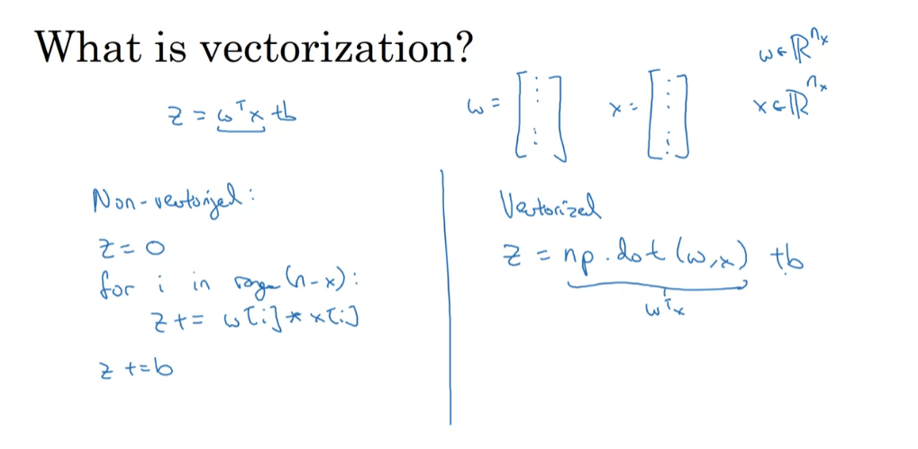
Let’s start with an example. So, what is Vectorization? In logistic regression you need to compute Z equals W transpose X plus B, where W was this column vector and X is also this vector. Maybe they are very large vectors if you have a lot of features. So, W and X were both these R and no R, NX dimensional vectors.

So, to compute W transpose X, if you had a non-vectorized implementation, you would do something like Z equals zero. And then for I in range of X. So, for I equals 1, 2 NX, Z plus equals W I times XI. And then maybe you do Z plus equal B at the end. So, that’s a non-vectorized implementation. Then you find that that’s going to be really slow.

In contrast, a vectorized implementation would just compute W transpose X directly. In Python or a numpy, the command you use for that is Z equals np.W, X, so this computes W transpose X. And you can also just add B to that directly. And you find that this is much faster.

Let’s actually illustrate this with a little demo. So, here’s my Jupiter notebook in which I’m going to write some Python code. So, first, let me import the numpy library to import. Send P. And so, for example, I can create A as an array as follows. Let’s say print A. Now, having written this chunk of code, if I hit shift enter, then it executes the code. So, it created the array A and it prints it out.

Vectorization version

Now, let’s do the Vectorization demo. I’m going to import the time libraries, since we use that, in order to time how long different operations take. Can they create an array A? Those random thought round. This creates a million dimensional array with random values. b = np.random.rand. Another million dimensional array. And, now, tic=time.time, so this measure the current time, c = np.dot (a, b). toc = time.time. And this print, it is the vectorized version.

It’s a vectorize version. And so, let’s print out. Let’s see the last time, so there’s toc - tic x 1000, so that we can express this in milliseconds. So, ms is milliseconds. I’m going to hit Shift Enter. So, that code took about three milliseconds or this time 1.5, maybe about 1.5 or 3.5 milliseconds at a time. It varies a little bit as I run it, but looks like maybe on average it’s taking like 1.5 milliseconds, maybe two milliseconds as I run this. All right. Let’s keep adding to this block of code.

Non-vectorized version

That’s not implementing non-vectorize version. Let’s see, c = 0, then tic = time.time. Now, let’s implement a for loop. For I in range of 1 million, I’ll pick out the number of zeros right. C += (a,i) x (b, i), and then toc = time.time. Finally, print more than explicit full loop. The time it takes is this 1000 x toc - tic + “ms” to know that we’re doing this in milliseconds. Let’s do one more thing. Let’s just print out the value of C we compute it to make sure that it’s the same value in both cases. I’m going to hit shift enter to run this and check that out. In both cases, the vectorize version and the non-vectorize version computed the same values, as you know, 2.50 to 6.99, so on.

The vectorize version took 1.5 milliseconds. The explicit for loop and non-vectorize version took about 400, almost 500 milliseconds. The non-vectorize version took something like 300 times longer than the vectorize version. With this example you see that if only you remember to vectorize your code, your code actually runs over 300 times faster. Let’s just run it again. Just run it again. Yeah. Vectorize version 1.5 milliseconds seconds and the for loop. So 481 milliseconds, again, about 300 times slower to do the explicit for loop.

If the engine x slows down, it’s the difference between your code taking maybe one minute to run versus taking say five hours to run. And when you are implementing deep learning algorithms, you can really get a result back faster. It will be much faster if you vectorize your code. Some of you might have heard that a lot of scaleable deep learning implementations are done on a GPU or a graphics processing unit. But all the demos I did just now in the Jupiter notebook where actually on the CPU. And it turns out that both GPU and CPU have parallelization instructions. They’re sometimes called SIMD instructions. This stands for a single instruction multiple data.

But what this basically means is that, if you use built-in functions such as this np.function or other functions that don’t require you explicitly implementing a for loop. It enables Python numpy to take much better advantage of parallelism to do your computations much faster. And this is true both computations on CPUs and computations on GPUs. It’s just that GPUs are remarkably good at these SIMD calculations but CPU is actually also not too bad at that. Maybe just not as good as GPUs.

You’re seeing how vectorization can significantly speed up your code. The rule of thumb to remember is whenever possible, avoid using explicit for loops. Let’s go onto the next video to see some more examples of vectorization and also start to vectorize logistic regression.

More Vectorization Examples

In the previous video you saw a few
examples of how vectorization, by using built in functions and
by avoiding explicit for loops, allows you to speed
up your code significantly. Let’s look at a few more examples. The rule of thumb to keep in mind is, when
you’re programming your neural networks, or when you’re programming just a regression, whenever possible avoid
explicit for-loops. And it’s not always possible to never
use a for-loop, but when you can use a built in function or find some
other way to compute whatever you need, you’ll often go faster than if
you have an explicit for-loop.

Let’s look at another example. If ever you want to compute a vector
u as the product of the matrix A, and another vector v,
then the definition of our matrix multiply is that your Ui is
equal to sum over j, Aij, Vj. That’s how you define Ui. And so
the non-vectorized implementation of this would be to set u equals NP.zeros,
it would be n by 1. For i, and so on. For j, and so on… And then u[i] plus equals
a[i][j] times v[j]. So now, this is two for-loops,
looping over both i and j.

So, that’s a non-vectorized version, the vectorized implementation which
is to say u equals np dot (A,v). And the implementation on the right,
the vectorized version, now eliminates two different for-loops,
and it’s going to be way faster.

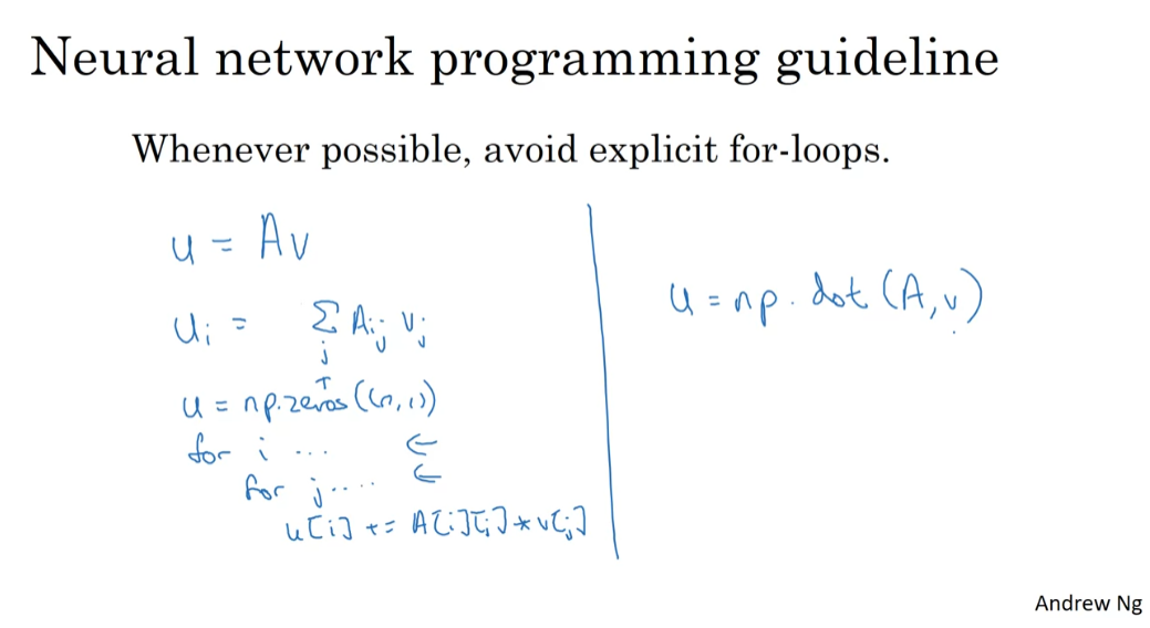
Let’s go through one more example. Let’s say you already have a vector,
v, in memory and you want to apply the exponential operation
on every element of this vector v. So you can put u equals the vector,
that’s e to the v1, e to the v2, and so on,
down to e to the vn. So this would be
a non-vectorized implementation, which is at first you initialize
u to the vector of zeros. And then you have a for-loop that
computes the elements one at a time.

But it turns out that Python and NumPy
have many built-in functions that allow you to compute these vectors with just
a single call to a single function. So what I would do to
implement this is import numpy as np, and then what you just call u = np.exp(v). And so, notice that, whereas previously
you had that explicit for-loop, with just one line of code here, just v
as an input vector u as an output vector, you’ve gotten rid of the explicit
for-loop, and the implementation on the right will be much faster that
the one needing an explicit for-loop.

In fact, the NumPy library has many
of the vector value functions. So np.log (v) will compute
the element-wise log, np.abs computes the absolute value, np.maximum computes
the element-wise maximum to take the max of every
element of v with 0. v**2 just takes the element-wise
square of each element of v. One over v takes the element-wise inverse,
and so on.

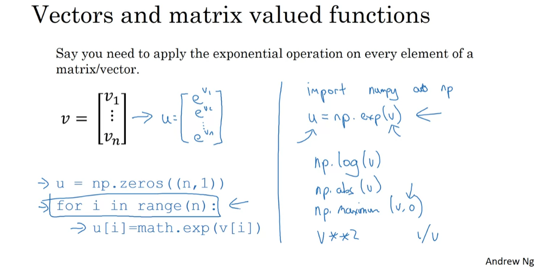
So, whenever you are tempted to write
a for-loop take a look, and see if there’s a way to call a NumPy built-in function
to do it without that for-loop. So, let’s take all of these learnings and apply it to our logistic regression
gradient descent implementation, and see if we can at least get rid
of one of the two for-loops we had.

So here’s our code for computing the derivatives for logistic
regression, and we had two for-loops. One was this one up here, and
the second one was this one. So in our example we had nx equals 2, but if you had more features than
just 2 features then you’d need have a for-loop over dw1,
dw2, dw3, and so on. So its as if there’s actually
a 4j equals 1, 2, and x. dWj gets updated. So we’d like to eliminate
this second for-loop. That’s what we’ll do on this slide. So the way we’ll do so
is that instead of explicitly initializing dw1, dw2, and so on to zeros, we’re going to get rid of this and
instead make dw a vector.

So we’re going to set dw equals np.zeros,
and let’s make this a nx by 1,
dimensional vector. Then, here, instead of this for loop over the individual components, we’ll just use this
vector value operation, dw plus equals xi times dz(i).

And then finally, instead of this, we will just have dw divides equals m. So now we’ve gone from having two
for-loops to just one for-loop. We still have this one for-loop that loops
over the individual training examples.

So I hope this video gave you
a sense of vectorization. And by getting rid of one for-loop
your code will already run faster. But it turns out we could do even better. So the next video will talk about how
to vectorize logistic aggression even further. And you see a pretty surprising result,
that without using any for-loops, without needing a for-loop
over the training examples, you could write code to process
the entire training sets. So, pretty much all at the same time. So, let’s see that in the next video.

Vectorizing Logistic Regression

vectorize the implementation of logistic regression

We have talked about how vectorization lets you speed up your code significantly. In this video, we’ll talk about how you can vectorize the implementation of logistic regression, so they can process an entire training set, that is implement a single elevation of grading descent with respect to an entire training set without using even a single explicit for loop. I’m super excited about this technique, and when we talk about neural networks later without using even a single explicit for loop.

Let’s get started. Let’s first examine the four propagation steps of logistic regression. So, if you have M training examples, then to make a prediction on the first example, you need to compute that, compute Z. I’m using this familiar formula, then compute the activations, you compute y hat in the first example. Then to make a prediction on the second training example, you need to compute that. Then, to make a prediction on the third example, you need to compute that, and so on. And you might need to do this M times, if you have M training examples.

X is a NX by M dimensional matrix.

So, it turns out, that in order to carry out the four propagation step, that is to compute these predictions on our M training examples, there is a way to do so, without needing an explicit for loop. Let’s see how you can do it. First, remember that we defined a matrix capital X to be your training inputs, stacked together in different columns like this. So, this is a matrix, that is a NX by M matrix. So, I’m writing this as a Python numpy shape, this just means that X is a NX by M dimensional matrix.

Now, the first thing I want to do is show how you can compute Z1, Z2, Z3 and so on, all in one step, in fact, with one line of code. So, I’m going to construct a 1 by M matrix that’s really a row vector while I’m going to compute Z1, Z2, and so on, down to ZM, all at the same time. It turns out that this can be expressed as W transpose to capital matrix X plus and then this vector B, B and so on. B, where this thing, this B, B, B, B, B thing is a 1xM vector or 1xM matrix or that is as a M dimensional row vector.

So hopefully there you are with matrix multiplication. You might see that W transpose X1, X2 and so on to XM, that W transpose can be a row vector. So this W transpose will be a row vector like that. And so this first term will evaluate to W transpose X1, W transpose X2 and so on, dot, dot, dot, W transpose XM, and then we add this second term B, B, B, and so on, you end up adding B to each element. So you end up with another 1xM vector. Well that’s the first element, that’s the second element and so on, and that’s the nth element.

And if you refer to the definitions above, this first element is exactly the definition of Z1. The second element is exactly the definition of Z2 and so on. So just as X was once obtained, when you took your training examples and stacked them next to each other, stacked them horizontally. I’m going to define capital Z to be this where you take the lowercase Z’s and stack them horizontally.

So when you stack the lower case X’s corresponding to a different training examples, horizontally you get this variable capital X and the same way when you take these lowercase Z variables, and stack them horizontally, you get this variable capital Z. And it turns out, that in order to implement this, the numpy command is capital Z equals NP dot W dot T, that’s W transpose X and then plus B. Now there is a subtlety in Python, which is at here B is a real number or if you want to say you know 1x1 matrix, is just a normal real number.

broadcasting

But, when you add this vector to this real number, Python automatically takes this real number B and expands it out to this 1XM row vector. So in case this operation seems a little bit mysterious, this is called broadcasting in Python, and you don’t have to worry about it for now, we’ll talk about it some more in the next video.

But the takeaway is that with just one line of code, with this line of code, you can calculate capital Z and capital Z is going to be a 1XM matrix that contains all of the lower cases Z’s. Lowercase Z1 through lower case ZM. So that was Z, how about these values A. What we like to do next, is find a way to compute A1, A2 and so on to AM, all at the same time, and just as stacking lowercase X’s resulted in capital X and stacking horizontally lowercase Z’s resulted in capital Z, stacking lower case A, is going to result in a new variable, which we are going to define as capital A.

And in the program assignment, you see how to implement a vector valued sigmoid function, so that the sigmoid function, inputs this capital Z as a variable and very efficiently outputs capital A. So you see the details of that in the programming assignment.

So just to recap, what we’ve seen on this slide is that instead of needing to loop over M training examples to compute lowercase Z and lowercase A, one of the time, you can implement this one line of code, to compute all these Z’s at the same time. And then, this one line of code, with appropriate implementation of lowercase Sigma to compute all the lowercase A’s all at the same time.

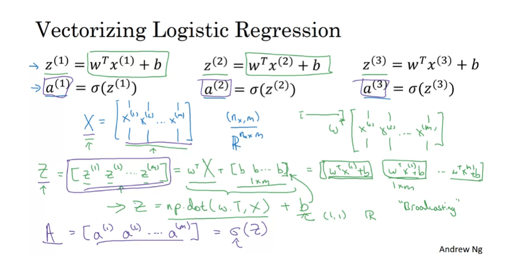
So this is how you implement a vectorize implementation of the four propagation for all M training examples at the same time. So to summarize, you’ve just seen how you can use vectorization to very efficiently compute all of the activations, all the lowercase A’s at the same time. Next, it turns out, you can also use vectorization very efficiently to compute the backward propagation, to compute the gradients. Let’s see how you can do that, in the next video.

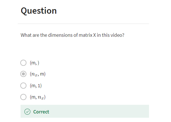
Vectorizing Logistic Regression’s Gradient Output

In the previous video, you saw how you can use vectorization to compute their predictions. The lowercase a’s for an entire training set all at the same time. In this video, you see how you can use vectorization to also perform the gradient computations for all M training samples. Again, all sort of at the same time. And then at the end of this video, we’ll put it all together and show how you can derive a very efficient implementation of logistic regression.

So, you may remember that for the gradient computation, what we did was we computed dz1 for the first example, which could be a1 minus y1 and then dz2 equals a2 minus y2 and so on. And so on for all M training examples. So, what we’re going to do is define a new variable, dZ is going to be dz1, dz2, dzm. Again, all the D lowercase z variables stacked horizontally. So, this would be 1 by m matrix or alternatively a m dimensional row vector.

Now recall that from the previous slide, we’d already figured out how to compute capital A which was this: a1 through am and we had defined capital Y as y1 through ym. Also you know, stacked horizontally. So, based on these definitions, maybe you can see for yourself that dz can be computed as just A minus Y because it’s going to be equal to a1 - y1. So, the first element, a2 - y2, so in the second element and so on.

And, so this first element a1 - y1 is exactly the definition of dz1. The second element is exactly the definition of dz2 and so on. So, with just one line of code, you can compute all of this at the same time. Now, in the previous implementation, we’ve gotten rid of one for loop already but we still had this second for loop over training examples.

So we initialize dw to zero to a vector of zeroes. But then we still have to loop over 20 examples where we have dw plus equals x1 times dz1, for the first training example dw plus equals x2 dz2 and so on. So we do the M times and then dw divide equals by M and similarly for B, right? db was initialized as 0 and db plus equals dz1. db plus equals dz2 down to you know dz(m) and db divide equals M. So that’s what we had in the previous implementation.

We’d already got rid of one for loop. So, at least now dw is a vector and we went separately updating dw1, dw2 and so on. So, we got rid of that already but we still had the for loop over the M examples in the training set. So, let’s take these operations and vectorize them. Here’s what we can do, for the vectorized implementation of db, what it’s doing is basically summing up, all of these dzs and then dividing by m.

So, db is basically one over m, sum from I equals one through m of dzi and well all the dzs are in that row vector and so in Python, what you do is implement you know, 1 over a m times np. sum of dz. So, you just take this variable and call the np. sum function on it and that would give you db. How about dw?

I’ll just write out the correct equations who can verify is the right thing to do. DW turns out to be one over M, times the matrix X times dz transpose. And, so kind of see why that’s the case. This is equal to one over m then the matrix X’s, x1 through xm stacked up in columns like that and dz transpose is going to be dz1 down to dz(m) like so. And so, if you figure out what this matrix times this vector works out to be, it is turns out to be one over m times x1 dz1 plus… plus xm dzm. And so, this is a n/1 vector and this is what you actually end up with, with dw because dw was taking these you know, xi dzi and adding them up and so that’s what exactly this matrix vector multiplication is doing and so again, with one line of code you can compute dw.

So, the vectorized implementation of the derivative calculations is just this, you use this line to implement db and use this line to implement dw and notice that without a for loop over the training set, you can now compute the updates you want to your parameters.

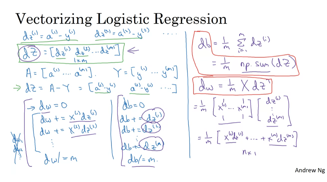
So now, let’s put all together into how you would actually implement logistic regression. So, this is our original, highly inefficient non vectorize implementation. So, the first thing we’ve done in the previous video was get rid of this volume, right? So, instead of looping over dw1, dw2 and so on, we have replaced this with a vector value dw which is dw+= xi, which is now a vector times dz(i). But now, we will see that we can also get rid of not just a for loop below but also get rid of this for loop.

So, here is how you do it. So, using what we have from the previous slides, you would say, capitalZ, Z equal to w transpose X + B and the code you is write capital Z equals np. w transpose X + B and then a equals sigmoid of capital Z. So, you have now computed all of this and all of this for all the values of I. Next on the previous slide, we said you would compute dz equals A - Y. So, now you computed all of this for all the values of i. Then, finally dw equals 1/m x dz transpose and db equals 1/m of you know, np. sum dz.

So, you’ve just done forward propagation and back propagation, really computing the predictions and computing the derivatives on all M training examples without using a for loop. And so the gradient descent update then would be you know W gets updated as w minus the learning rate times dw which was just computed above and B is update as B minus the learning rate times db. Sometimes is putting colons to that to denote that as is an assignment, but I guess I haven’t been totally consistent with that notation.

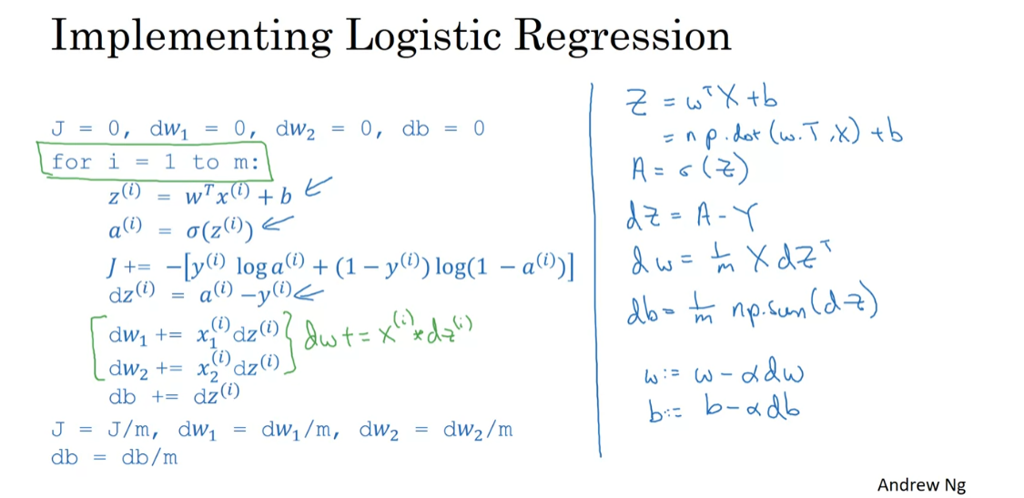
But with this, you have just implemented a single iteration of gradient descent for logistic regression. Now, I know I said that we should get rid of explicit for loops whenever you can but if you want to implement multiple iterations as a gradient descent then you still need a for loop over the number of iterations. So, if you want to have a thousand iterations of gradient descent, you might still need a for loop over the iteration number. There is an outermost for loop like that then I don’t think there is any way to get rid of that for loop.

But I do think it’s incredibly cool that you can implement at least one iteration of gradient descent without needing to use a for loop. So, that’s it you now have a highly vectorize and highly efficient implementation of gradient descent for logistic regression. There is just one more detail that I want to talk about in the next video, which is in our description here I briefly alluded to this technique called broadcasting. Broadcasting turns out to be a technique that Python and numpy allows you to use to make certain parts of your code also much more efficient. So, let’s see some more details of broadcasting in the next video.

Broadcasting in Python

In the previous video,
I mentioned that broadcasting is another technique that you can use
to make your Python code run faster. In this video, let’s delve into how
broadcasting in Python actually works. Let’s explore
broadcasting with an example. In this matrix, I’ve shown the number
of calories from carbohydrates, proteins, and
fats in 100 grams of four different foods. So for example,
a 100 grams of apples turns out, has 56 calories from carbs, and
much less from proteins and fats. Whereas, in contrast, a 100 grams of
beef has 104 calories from protein and 135 calories from fat.

Now, let’s say your goal is to
calculate the percentage of calories from carbs, proteins and
fats for each of the four foods. So, for example,
if you look at this column and add up the numbers in that column
you get that 100 grams of apple has 56 plus 1.2 plus 1.8 so
that’s 59 calories. And so as a percentage the percentage of calories from carbohydrates
in an apple would be 56 over 59, that’s about 94.9%. So most of the calories in an apple
come from carbs, whereas in contrast, most of the calories of beef come
from protein and fat and so on. So the calculation you want is really
to sum up each of the four columns of this matrix to get the total number
of calories in 100 grams of apples, beef, eggs, and potatoes. And then to divide throughout the matrix, so as to get the percentage of
calories from carbs, proteins and fats for each of the four foods.

So the question is, can you do
this without an explicit for-loop? Let’s take a look at
how you could do that. What I’m going to do is
show you how you can set, say this matrix equal to
three by four matrix A. And then with one line of Python code
we’re going to sum down the columns. So we’re going to get four numbers
corresponding to the total number of calories in these four
different types of foods, 100 grams of these four
different types of foods. And I’m going to use a second line
of Python code to divide each of the four columns by
their corresponding sum. If that verbal description
wasn’t very clearly, hopefully it will be clearer in a second
when we look in the Python code. So here we are in the Jupiter notebook. I’ve already written this first
piece of code to prepopulate the matrix A with the numbers we had
just now, so we’ll hit shift enter and just run that, so there’s the matrix A. And now here are the two
lines of Python code. First, we’re going to compute
tau equals a, that sum. And x is equals 0 means to sum vertically. We’ll say more about that in a little bit. And then print cal. So we’ll sum vertically. Now 59 is the total number of
calories in the apple, 239 was the total number of calories in the beef
and the eggs and potato and so on. And then with a compute percentage equals A/cal.reshape 1,4. Actually we want percentages,
so multiply by 100 here. And then let’s print percentage. Let’s run that. And so
that command we’ve taken the matrix A and divided it by this one by four matrix. And this gives us
the matrix of percentages. So as we worked out kind of by
hand just now in the apple there was a first column 94.9% of
the calories are from carbs.

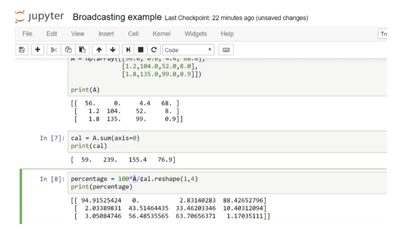
Let’s go back to the slides. So just to repeat the two
lines of code we had, this is what have written
out in the Jupiter notebook. To add a bit of detail this parameter, (axis = 0), means that you
want Python to sum vertically. So if this is axis 0 this
means to sum vertically, where as the horizontal axis is axis 1. So be able to write axis 1 or sum
horizontally instead of sum vertically. And then this command here, this is an example of Python
broadcasting where you take a matrix A. So this is a three by four matrix and
you divide it by a one by four matrix. And technically, after this first
line of codes cal, the variable cal, is already a one by four matrix. So technically you don’t need
to call reshape here again, so that’s actually a little bit redundant. But when I’m writing Python codes if
I’m not entirely sure what matrix, whether the dimensions of a matrix I often
would just call a reshape command just to make sure that it’s the right
column vector or the row vector or whatever you want it to be. The reshape command is a constant time. It’s a order one operation
that’s very cheap to call. So don’t be shy about using the reshape
command to make sure that your matrices are the size you need it to be.

Now, let’s explain in greater detail how
this type of operation works, right? We had a three by four matrix and
we divided it by a one by four matrix. So, how can you divide a three by
four matrix by a one by four matrix? Or by one by four vector?

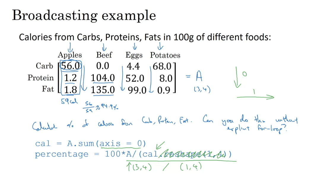
Let’s go through a few more
examples of broadcasting. If you take a 4 by 1 vector and
add it to a number, what Python will do is take this number and
auto-expand it into a four by one vector as well,
as follows. And so the vector [1, 2, 3, 4] plus the number 100 ends up
with that vector on the right. You’re adding a 100 to every element,
and in fact we use this form of broadcasting where that constant was
the parameter b in an earlier video. And this type of broadcasting works with
both column vectors and row vectors, and in fact we use a similar form of
broadcasting earlier with the constant we’re adding to a vector being
the parameter b in logistic regression.

Here’s another example. Let’s say you have a two
by three matrix and you add it to this one by n matrix. So the general case would be if you have some (m,n) matrix here and you add it to a (1,n) matrix. What Python will do is copy the matrix m, times to turn this into m by n matrix,
so instead of this one by three matrix it’ll copy it twice in
this example to turn it into this. Also, two by three matrix and
we’ll add these so you’ll end up with the sum on the right,
okay? So you taken,
you added 100 to the first column, added 200 to second column,
added 300 to the third column. And this is basically what we
did on the previous slide, except that we use a division operation
instead of an addition operation.

So one last example,
whether you have a (m,n) matrix and you add this to a (m,1) vector,
(m,1) matrix. Then just copy this n times horizontally. So you end up with an (m,n) matrix. So as you can imagine you copy
it horizontally three times. And you add those. So when you add them you end up with this. So we’ve added 100 to the first row and
added 200 to the second row.

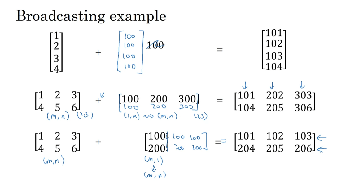
Here’s the more general principle
of broadcasting in Python. If you have an (m,n) matrix and you add or subtract or multiply or
divide with a (1,n) matrix, then this will copy it n
times into an (m,n) matrix. And then apply the addition,
subtraction, and multiplication of division element wise. If conversely, you were to take the (m,n)
matrix and add, subtract, multiply, divide by an (m,1) matrix,
then also this would copy it now n times. And turn that into an (m,n) matrix and
then apply the operation element wise. Just one of the broadcasting,
which is if you have an (m,1) matrix, so that’s really a column vector
like [1,2,3], and you add, subtract, multiply or
divide by a row number. So maybe a (1,1) matrix. So such as that plus 100,
then you end up copying this real number n times until you’ll
also get another (n,1) matrix. And then you perform the operation such
as addition on this example element-wise. And something similar also works for
row vectors.

The fully general version of broadcasting
can do even a little bit more than this. If you’re interested you can
read the documentation for NumPy, and look at broadcasting
in that documentation. That gives an even slightly more
general definition of broadcasting. But the ones on the slide are the main
forms of broadcasting that you end up needing to use when you
implement a neural network.

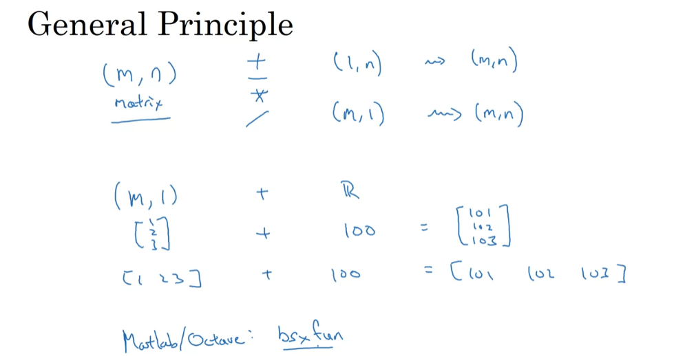
Before we wrap up,
just one last comment, which is for those of you that are used to
programming in either MATLAB or Octave, if you’ve ever used the MATLAB or
Octave function bsxfun in neural network programming bsxfun does
something similar, not quite the same. But it is often used for similar purpose
as what we use broadcasting in Python for. But this is really only for
very advanced MATLAB and Octave users, if you’ve not heard of this,
don’t worry about it. You don’t need to know it when you’re
coding up neural networks in Python. So, that was broadcasting in Python. I hope that when you do the programming
homework that broadcasting will allow you to not only make a code run faster, but also help you get what you want
done with fewer lines of code. Before you dive into the programming
excercise, I want to share with you just one more set of ideas,
which is that there’s some tips and tricks that I’ve found reduces
the number of bugs in my Python code and that I hope will help you too. So with that,
let’s talk about that in the next video.

A Note on Python/Numpy Vectors

The ability of python to allow you
to use broadcasting operations and more generally, the great flexibility of
the python numpy program language is, I think, both a strength as well as
a weakness of the programming language. I think it’s a strength because they
create expressivity of the language. A great flexibility of the language lets
you get a lot done even with just a single line of code. But there’s also weakness because with
broadcasting and this great amount of flexibility, sometimes it’s possible
you can introduce very subtle bugs or very strange looking bugs, if you’re not
familiar with all of the intricacies of how broadcasting and
how features like broadcasting work.

For example, if you take a column vector
and add it to a row vector, you would expect it to throw up a dimension
mismatch or type error or something. But you might actually get back
a matrix as a sum of a row vector and a column vector. So there is an internal logic to
these strange effects of Python. But if you’re not familiar with Python,
I’ve seen some students have very strange, very hard to find bugs. So what I want to do in this video is
share with you some couple tips and tricks that have been very useful for
me to eliminate or simplify and eliminate all the strange
looking bugs in my own code. And I hope that with these tips and
tricks, you’ll also be able to much more easily
write bug-free, python and numpy code.

suggestions on python code

To illustrate one of the less
intuitive effects of Python-Numpy, especially how you construct vectors in
Python-Numpy, let me do a quick demo. Let’s set a = np.random.randn(5), so this creates five random Gaussian variables stored in array a. And so let’s print(a) and
now it turns out that the shape of a when you do this
is this five comma structure. And so this is called a rank
1 array in Python and it’s neither a row vector nor
a column vector. And this leads it to have some
slightly non-intuitive effects. So for example, if I print a transpose,
it ends up looking the same as a. So a and
a transpose end up looking the same. And if I print the inner product between
a and a transpose, you might think a times a transpose is maybe the outer
product should give you matrix maybe. But if I do that,
you instead get back a number. So what I would recommend is that
when you’re coding new networks, that you just not use data structures
where the shape is 5, or n, rank 1 array.

Instead, if you set a to be this, (5,1), then this commits a to
be (5,1) column vector. And whereas previously, a and
a transpose looked the same, it becomes now a transpose,
now a transpose is a row vector. Notice one subtle difference. In this data structure, there are two
square brackets when we print a transpose. Whereas previously,
there was one square bracket. So that’s the difference
between this is really a 1 by 5 matrix versus one of
these rank 1 arrays. And if you print, say,
the product between a and a transpose, then this gives you the outer
product of a vector, right? And so, the outer product of
a vector gives you a matrix.

So, let’s look in greater detail
at what we just saw here. The first command that we ran,
just now, was this. And this created a data structure with a.shape was this funny thing (5,) so this is called a rank 1 array. And this is a very funny data structure. It doesn’t behave consistently as either
a row vector nor a column vector, which makes some of its
effects nonintuitive. So what I’m going to recommend is that
when you’re doing your programing exercises, or in fact when you’re
implementing logistic regression or neural networks that you just
do not use these rank 1 arrays.

Instead, if every time
you create an array, you commit to making it
either a column vector, so this creates a (5,1) vector, or
commit to making it a row vector, then the behavior of your vectors
may be easier to understand. So in this case,
a.shape is going to be equal to 5,1. And so this behaves a lot like a, but
in fact, this is a column vector. And that’s why you can think of this as
(5,1) matrix, where it’s a column vector. And here a.shape is going to be 1,5, and this behaves consistently
as a row vector. So when you need a vector,
I would say either use this or this, but not a rank 1 array.

One more thing that I do a lot in my
code is if I’m not entirely sure what’s the dimension of one of my vectors,
I’ll often throw in an assertion statement like this, to make sure, in this case,
that this is a (5,1) vector. So this is a column vector. These assertions are really
inexpensive to execute, and they also help to serve as
documentation for your code. So don’t hesitate to throw in assertion
statements like this whenever you feel like.

And then finally, if for some reason
you do end up with a rank 1 array, You can reshape this, a equals a.reshape into say a (5,1) array or a (1,5) array so that it behaves more consistently as
either column vector or row vector. So I’ve sometimes seen students
end up with very hard to track because those are the nonintuitive
effects of rank 1 arrays. By eliminating rank 1 arrays in my old
code, I think my code became simpler. And I did not actually find it
restrictive in terms of things I could express in code. I just never used a rank 1 array.

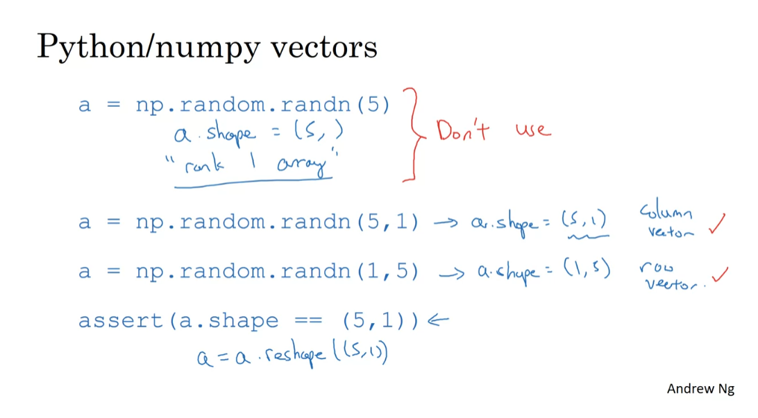
And so takeaways are to simplify
your code, don’t use rank 1 arrays. Always use either n by one matrices, basically column vectors, or one by
n matrices, or basically row vectors. Feel free to toss a lot of
insertion statements, so double-check the dimensions
of your matrices and arrays. And also, don’t be shy about calling the
reshape operation to make sure that your matrices or your vectors
are the dimension that you need it to be. So that, I hope that this set of suggestions
helps you to eliminate a cause of bugs from Python code, and makes the problem
exercise easier for you to complete.

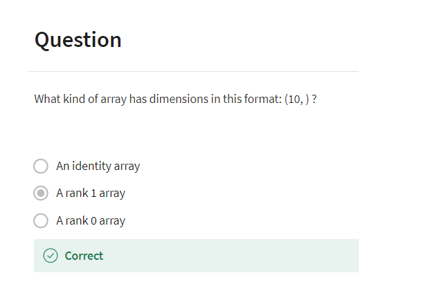
[3] Quiz: Neural Network Basics

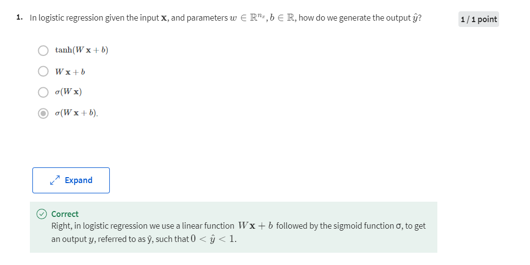
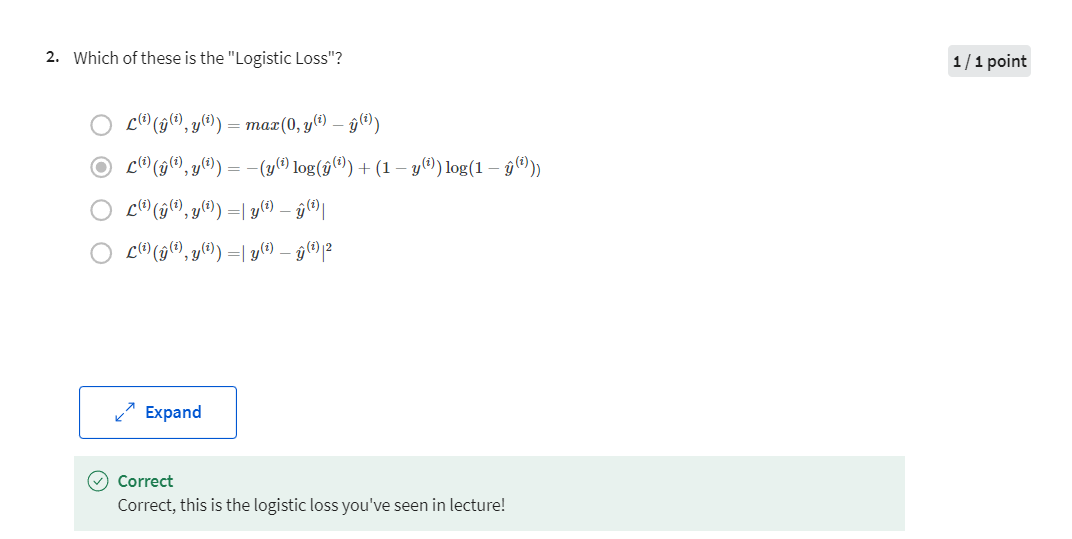
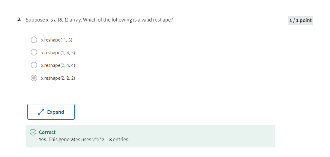
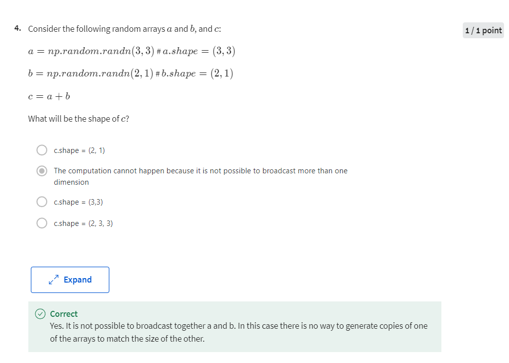
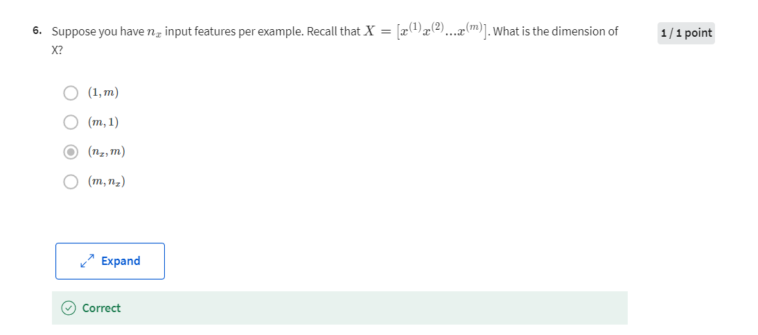
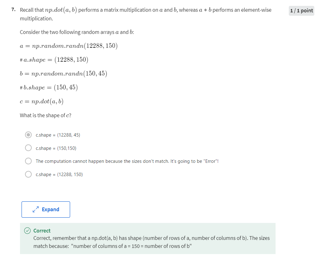
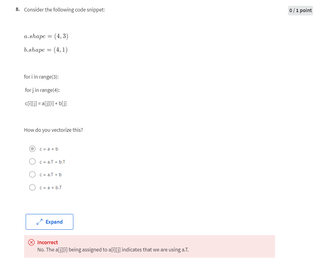
这题应该 选 a.T + b.T

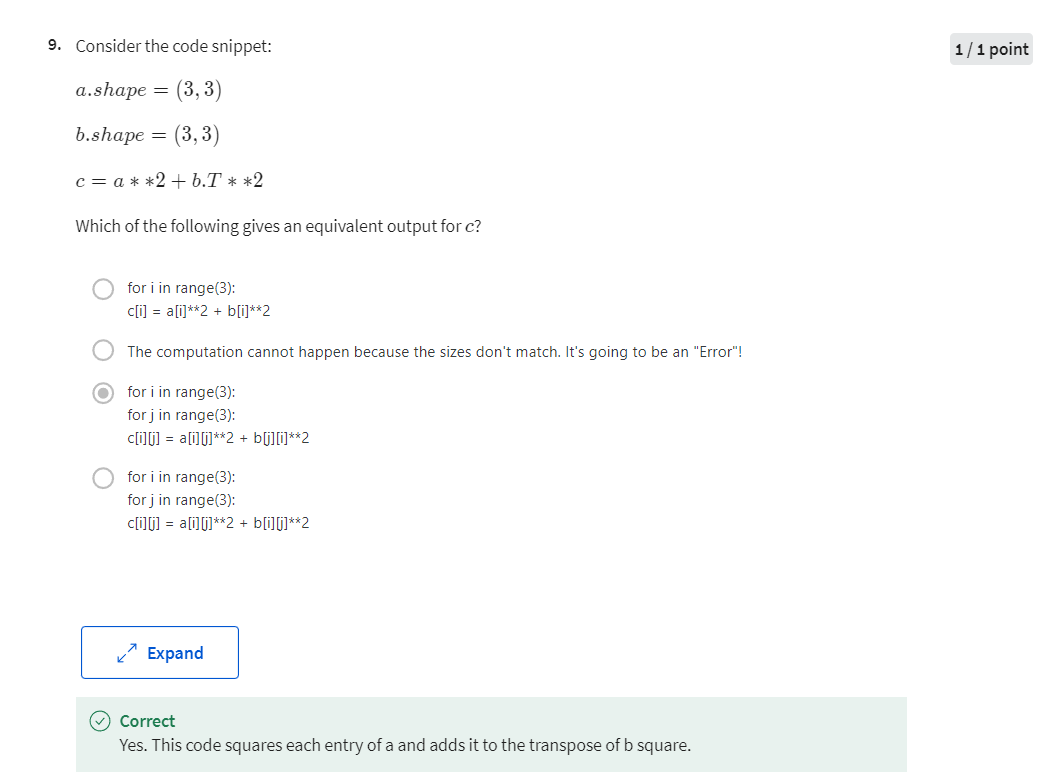
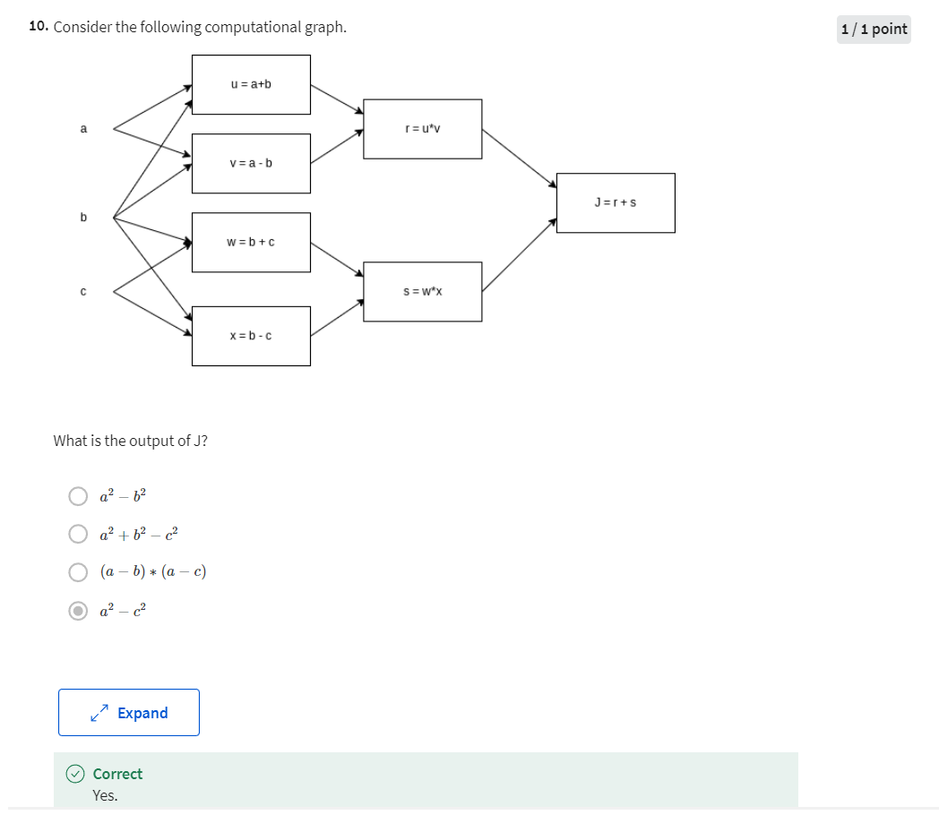
Programming Assignment: Python Basics with Numpy (optional assignment)

Welcome to your first assignment. This exercise gives you a brief introduction to Python. Even if you’ve used Python before, this will help familiarize you with the functions we’ll need.

Instructions:

• You will be using Python 3.
• Avoid using for-loops and while-loops, unless you are explicitly told to do so.
• After coding your function, run the cell right below it to check if your result is correct.

After this assignment you will:

• Be able to use iPython Notebooks
• Be able to use numpy functions and numpy matrix/vector operations
• Understand the concept of “broadcasting”
• Be able to vectorize code

Let’s get started!

Important Note on Submission to the AutoGrader

Before submitting your assignment to the AutoGrader, please make sure you are not doing the following:

1. You have not added any extra print statement(s) in the assignment.
2. You have not added any extra code cell(s) in the assignment.
3. You have not changed any of the function parameters.
4. You are not using any global variables inside your graded exercises. Unless specifically instructed to do so, please refrain from it and use the local variables instead.
5. You are not changing the assignment code where it is not required, like creating extra variables.

If you do any of the following, you will get something like, Grader Error: Grader feedback not found (or similarly unexpected) error upon submitting your assignment. Before asking for help/debugging the errors in your assignment, check for these first. If this is the case, and you don’t remember the changes you have made, you can get a fresh copy of the assignment by following these instructions.

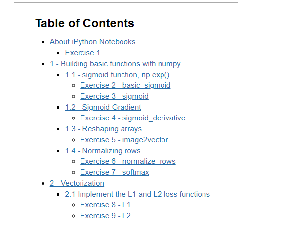
Exercise 1

Set test to "Hello World" in the cell below to print “Hello World” and run the two cells below.

# (≈ 1 line of code)
# test = 
# YOUR CODE STARTS HERE
test = "Hello World"
# YOUR CODE ENDS HERE

print ("test: " + test)

Output

test: Hello World

Expected output:
test: Hello World

1 - Building basic functions with numpy

Numpy is the main package for scientific computing in Python. It is maintained by a large community (www.numpy.org). In this exercise you will learn several key numpy functions such as np.exp, np.log, and np.reshape. You will need to know how to use these functions for future assignments.

1.1 - sigmoid function, np.exp()

Before using np.exp(), you will use math.exp() to implement the sigmoid function. You will then see why np.exp() is preferable to math.exp().

Exercise 2 - basic_sigmoid

Build a function that returns the sigmoid of a real number x. Use math.exp(x) for the exponential function.

Reminder:
$sigmoid(x)=\frac{1}{1+e^{-x}}$ is sometimes also known as the logistic function. It is a non-linear function used not only in Machine Learning (Logistic Regression), but also in Deep Learning.

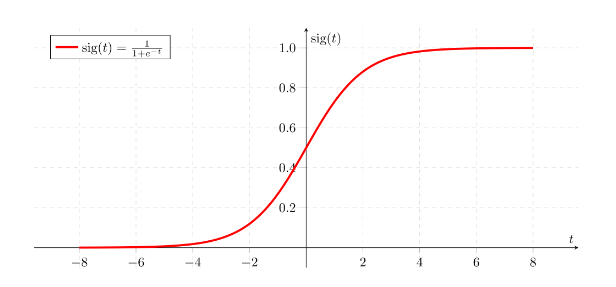
To refer to a function belonging to a specific package you could call it using package_name.function(). Run the code below to see an example with math.exp().

import math
from public_tests import *

# GRADED FUNCTION: basic_sigmoid

def basic_sigmoid(x):
    """
    Compute sigmoid of x.

    Arguments:
    x -- A scalar

    Return:
    s -- sigmoid(x)
    """
    # (≈ 1 line of code)
    # s = 
    # YOUR CODE STARTS HERE
    s = 1 / (1 + math.exp(-x))
    
    # YOUR CODE ENDS HERE
    
    return s

print("basic_sigmoid(1) = " + str(basic_sigmoid(1)))

basic_sigmoid_test(basic_sigmoid)

Output

basic_sigmoid(1) = 0.7310585786300049
 All tests passed.

Actually, we rarely use the “math” library in deep learning because the inputs of the functions are real numbers. In deep learning we mostly use matrices and vectors. This is why numpy is more useful.

### One reason why we use "numpy" instead of "math" in Deep Learning ###

x = [1, 2, 3] # x becomes a python list object
basic_sigmoid(x) # you will see this give an error when you run it, because x is a vector.

In fact, if $ x = (x_1, x_2, …, x_n)$ is a row vector then np.exp(x) will apply the exponential function to every element of x. The output will thus be: np.exp(x) = (e^{x_1}, e^{x_2}, ..., e^{x_n})

import numpy as np

# example of np.exp
t_x = np.array([1, 2, 3])
print(np.exp(t_x)) # result is (exp(1), exp(2), exp(3))

Output

[ 2.71828183  7.3890561  20.08553692]

Furthermore, if x is a vector, then a Python operation such as $s=x+3$ or $s=\frac{1}{x}$ will output s as a vector of the same size as x.

# example of vector operation
t_x = np.array([1, 2, 3])
print (t_x + 3)

Output

[4 5 6]

Any time you need more info on a numpy function, we encourage you to look at the official documentation.

You can also create a new cell in the notebook and write np.exp? (for example) to get quick access to the documentation.

Exercise 3 - sigmoid

Implement the sigmoid function using numpy.

Instructions: x could now be either a real number, a vector, or a matrix. The data structures we use in numpy to represent these shapes (vectors, matrices…) are called numpy arrays. You don’t need to know more for now.
$$\text{For }x\in {\mathbb{R}}^n\text{, }sigmoid(x)=sigmoid\left(\begin{array}{c}{x}_1\\ x_2\\ ...\\ x_n\end{array}\right)=\left(\begin{array}{c}\frac{1}{1+e^{-x_1}}\\ \frac{1}{1+e^{-x_2}}\\ ...\\ \frac{1}{1+e^{-x_n}}\end{array}\right)\text{\hspace{1em}(1)}$$

# GRADED FUNCTION: sigmoid

def sigmoid(x):
    """
    Compute the sigmoid of x

    Arguments:
    x -- A scalar or numpy array of any size

    Return:
    s -- sigmoid(x)
    """
    
    # (≈ 1 line of code)
    # s = 
    # YOUR CODE STARTS HERE
    
    s = 1 / (1 + np.exp(-x))
    # YOUR CODE ENDS HERE
    
    return s

t_x = np.array([1, 2, 3])
print("sigmoid(t_x) = " + str(sigmoid(t_x)))

sigmoid_test(sigmoid)

Output

sigmoid(t_x) = [0.73105858 0.88079708 0.95257413]
 All tests passed.

1.2 - Sigmoid Gradient

As you’ve seen in lecture, you will need to compute gradients to optimize loss functions using backpropagation. Let’s code your first gradient function.

Exercise 4 - sigmoid_derivative

Implement the function sigmoid_grad() to compute the gradient of the sigmoid function with respect to its input x. The formula is:

$$sigmoid\_derivative(x)={\sigma }^{\prime }(x)=\sigma (x)(1-\sigma (x))\text{\hspace{1em}(2)}$$

You often code this function in two steps:

1. Set s to be the sigmoid of x. You might find your sigmoid(x) function useful.
2. Compute ${\sigma }^{\prime }(x)=s(1-s)$

# GRADED FUNCTION: sigmoid_derivative

def sigmoid_derivative(x):
    """
    Compute the gradient (also called the slope or derivative) of the sigmoid function with respect to its input x.
    You can store the output of the sigmoid function into variables and then use it to calculate the gradient.
    
    Arguments:
    x -- A scalar or numpy array

    Return:
    ds -- Your computed gradient.
    """
    
    #(≈ 2 lines of code)
    # s = 
    # ds = 
    # YOUR CODE STARTS HERE
    s = sigmoid(x)
    ds = s * (1 - s)
    
    # YOUR CODE ENDS HERE
    
    return ds

t_x = np.array([1, 2, 3])
print ("sigmoid_derivative(t_x) = " + str(sigmoid_derivative(t_x)))

sigmoid_derivative_test(sigmoid_derivative)

Output

sigmoid_derivative(t_x) = [0.19661193 0.10499359 0.04517666]
 All tests passed.

1.3 - Reshaping arrays

Two common numpy functions used in deep learning are np.shape and np.reshape().

• X.shape is used to get the shape (dimension) of a matrix/vector X.
• X.reshape(…) is used to reshape X into some other dimension.

For example, in computer science, an image is represented by a 3D array of shape $(length,height,depth=3)$. However, when you read an image as the input of an algorithm you convert it to a vector of shape $(length\ast height\ast 3,1)$. In other words, you “unroll”, or reshape, the 3D array into a 1D vector.

Exercise 5 - image2vector

Implement image2vector() that takes an input of shape (length, height, 3) and returns a vector of shape (length*height*3, 1). For example, if you would like to reshape an array v of shape (a, b, c) into a vector of shape (a*b,c) you would do:

v = v.reshape((v.shape[0] * v.shape[1], v.shape[2])) # v.shape[0] = a ; v.shape[1] = b ; v.shape[2] = c

• Please don’t hardcode the dimensions of image as a constant. Instead look up the quantities you need with image.shape[0], etc.
• You can use v = v.reshape(-1, 1). Just make sure you understand why it works.

# GRADED FUNCTION:image2vector

def image2vector(image):
    """
    Argument:
    image -- a numpy array of shape (length, height, depth)
    
    Returns:
    v -- a vector of shape (length*height*depth, 1)
    """
    
    # (≈ 1 line of code)
    # v =
    # YOUR CODE STARTS HERE
    v = image.reshape(image.shape[0] * image.shape[1] * image.shape[2], 1)
    
    # YOUR CODE ENDS HERE
    
    return v

# This is a 3 by 3 by 2 array, typically images will be (num_px_x, num_px_y,3) where 3 represents the RGB values
t_image = np.array([[[ 0.67826139,  0.29380381],
                     [ 0.90714982,  0.52835647],
                     [ 0.4215251 ,  0.45017551]],

                   [[ 0.92814219,  0.96677647],
                    [ 0.85304703,  0.52351845],
                    [ 0.19981397,  0.27417313]],

                   [[ 0.60659855,  0.00533165],
                    [ 0.10820313,  0.49978937],
                    [ 0.34144279,  0.94630077]]])

print ("image2vector(image) = " + str(image2vector(t_image)))

image2vector_test(image2vector)

Output

image2vector(image) = [[0.67826139]
 [0.29380381]
 [0.90714982]
 [0.52835647]
 [0.4215251 ]
 [0.45017551]
 [0.92814219]
 [0.96677647]
 [0.85304703]
 [0.52351845]
 [0.19981397]
 [0.27417313]
 [0.60659855]
 [0.00533165]
 [0.10820313]
 [0.49978937]
 [0.34144279]
 [0.94630077]]
 All tests passed.

1.4 - Normalizing rows

Another common technique we use in Machine Learning and Deep Learning is to normalize our data. It often leads to a better performance because gradient descent converges faster after normalization. Here, by normalization we mean changing x to $ \frac{x}{| x|} $ (dividing each row vector of x by its norm).

For example, if
$$x=\left[\begin{array}{ccc}0& 3& 4\\ 2& 6& 4\end{array}\right]\text{\hspace{1em}(3)}$$
then
$$\Vert x\Vert =\text{np.linalg.norm(x, axis=1, keepdims=True)}=\left[\begin{array}{c}5\\ \sqrt{56}\end{array}\right]\text{\hspace{1em}(4)}$$
and
$$x\_normalized=\frac{x}{\Vert x\Vert }=\left[\begin{array}{ccc}0& \frac{3}{5}& \frac{4}{5}\\ \frac{2}{\sqrt{56}}& \frac{6}{\sqrt{56}}& \frac{4}{\sqrt{56}}\end{array}\right]\text{\hspace{1em}(5)}$$

Note that you can divide matrices of different sizes and it works fine: this is called broadcasting and you’re going to learn about it in part 5.

With keepdims=True the result will broadcast correctly against the original x.

axis=1 means you are going to get the norm in a row-wise manner. If you need the norm in a column-wise way, you would need to set axis=0.

numpy.linalg.norm has another parameter ord where we specify the type of normalization to be done (in the exercise below you’ll do 2-norm). To get familiar with the types of normalization you can visit numpy.linalg.norm

Exercise 6 - normalize_rows

Implement normalizeRows() to normalize the rows of a matrix. After applying this function to an input matrix x, each row of x should be a vector of unit length (meaning length 1).

# GRADED FUNCTION: normalize_rows

def normalize_rows(x):
    """
    Implement a function that normalizes each row of the matrix x (to have unit length).
    
    Argument:
    x -- A numpy matrix of shape (n, m)
    
    Returns:
    x -- The normalized (by row) numpy matrix. You are allowed to modify x.
    """
    
    #(≈ 2 lines of code)
    # Compute x_norm as the norm 2 of x. Use np.linalg.norm(..., ord = 2, axis = ..., keepdims = True)
    # x_norm =
    # Divide x by its norm.
    # x =
    # YOUR CODE STARTS HERE
    x_norm = np.linalg.norm(x, ord = 2, axis=1, keepdims=True)
    x /= x_norm
    
    # YOUR CODE ENDS HERE

    return x

x = np.array([[0., 3., 4.],
              [1., 6., 4.]])
print("normalizeRows(x) = " + str(normalize_rows(x)))

normalizeRows_test(normalize_rows)

Output

normalizeRows(x) = [[0.         0.6        0.8       ]
 [0.13736056 0.82416338 0.54944226]]
 All tests passed.

Note:
In normalize_rows(), you can try to print the shapes of x_norm and x, and then rerun the assessment. You’ll find out that they have different shapes. This is normal given that x_norm takes the norm of each row of x. So x_norm has the same number of rows but only 1 column. So how did it work when you divided x by x_norm? This is called broadcasting and we’ll talk about it now!

Exercise 7 - softmax

Implement a softmax function using numpy. You can think of softmax as a normalizing function used when your algorithm needs to classify two or more classes. You will learn more about softmax in the second course of this specialization.

Instructions:

• $\text{for }x\in {\mathbb{R}}^{1\times n}\text{, }$

$$\begin{array}{rl}softmax(x)& =softmax\left(\left[\begin{array}{ccccccc}{x}_1& & x_2& & ...& & x_n\end{array}\right]\right)\\ & =\left[\begin{array}{ccccccc}\frac{e^{x_1}}{{\sum }_j{e}^{x_j}}& & \frac{e^{x_2}}{{\sum }_j{e}^{x_j}}& & ...& & \frac{e^{x_n}}{{\sum }_j{e}^{x_j}}\end{array}\right]\end{array}$$

• $$\text{for a matrix }x\in {\mathbb{R}}^{m\times n}\text{, xij maps to the element in the ith row and jth column of x, thus we have: }$$

$$\begin{array}{rl}softmax(x)& =softmax\left[\begin{array}{ccccc}{x}_{11}& x_{12}& x_{13}& \dots & x_{1n}\\ x_{21}& x_{22}& x_{23}& \dots & x_{2n}\\ ⋮& ⋮& ⋮& \ddots & ⋮\\ x_{m1}& x_{m2}& x_{m3}& \dots & x_{mn}\end{array}\right]\\ & \\ & =\left[\begin{array}{ccccc}\frac{e^{x_{11}}}{{\sum }_j{e}^{x_{1j}}}& \frac{e^{x_{12}}}{{\sum }_j{e}^{x_{1j}}}& \frac{e^{x_{13}}}{{\sum }_j{e}^{x_{1j}}}& \dots & \frac{e^{x_{1n}}}{{\sum }_j{e}^{x_{1j}}}\\ \frac{e^{x_{21}}}{{\sum }_j{e}^{x_{2j}}}& \frac{e^{x_{22}}}{{\sum }_j{e}^{x_{2j}}}& \frac{e^{x_{23}}}{{\sum }_j{e}^{x_{2j}}}& \dots & \frac{e^{x_{2n}}}{{\sum }_j{e}^{x_{2j}}}\\ ⋮& ⋮& ⋮& \ddots & ⋮\\ \frac{e^{x_{m1}}}{{\sum }_j{e}^{x_{mj}}}& \frac{e^{x_{m2}}}{{\sum }_j{e}^{x_{mj}}}& \frac{e^{x_{m3}}}{{\sum }_j{e}^{x_{mj}}}& \dots & \frac{e^{x_{mn}}}{{\sum }_j{e}^{x_{mj}}}\end{array}\right]\\ & \\ & =\left(\begin{array}{c}softmax\text{(first row of x)}\\ softmax\text{(second row of x)}\\ ⋮\\ softmax\text{(last row of x)}\end{array}\right)\end{array}$$

Notes:
Note that later in the course, you’ll see “m” used to represent the “number of training examples”, and each training example is in its own column of the matrix. Also, each feature will be in its own row (each row has data for the same feature).
Softmax should be performed for all features of each training example, so softmax would be performed on the columns (once we switch to that representation later in this course).

However, in this coding practice, we’re just focusing on getting familiar with Python, so we’re using the common math notation $m\times n$
where $m$ is the number of rows and $n$ is the number of columns.

# GRADED FUNCTION: softmax

def softmax(x):
    """Calculates the softmax for each row of the input x.

    Your code should work for a row vector and also for matrices of shape (m,n).

    Argument:
    x -- A numpy matrix of shape (m,n)

    Returns:
    s -- A numpy matrix equal to the softmax of x, of shape (m,n)
    """
    
    #(≈ 3 lines of code)
    # Apply exp() element-wise to x. Use np.exp(...).
    # x_exp = ...

    # Create a vector x_sum that sums each row of x_exp. Use np.sum(..., axis = 1, keepdims = True).
    # x_sum = ...
    
    # Compute softmax(x) by dividing x_exp by x_sum. It should automatically use numpy broadcasting.
    # s = ...
    
    # YOUR CODE STARTS HERE
    
    x_exp = np.exp(x)
    x_sum = np.sum(x_exp, axis=1, keepdims=True)
    s = x_exp / x_sum
    
    # YOUR CODE ENDS HERE
    
    return s

t_x = np.array([[9, 2, 5, 0, 0],
                [7, 5, 0, 0 ,0]])
print("softmax(x) = " + str(softmax(t_x)))

softmax_test(softmax)

Output

softmax(x) = [[9.80897665e-01 8.94462891e-04 1.79657674e-02 1.21052389e-04
  1.21052389e-04]
 [8.78679856e-01 1.18916387e-01 8.01252314e-04 8.01252314e-04
  8.01252314e-04]]
 All tests passed.

Notes

• If you print the shapes of x_exp, x_sum and s above and rerun the assessment cell, you will see that x_sum is of shape (2,1) while x_exp and s are of shape (2,5). x_exp/x_sum works due to python broadcasting.

Congratulations! You now have a pretty good understanding of python numpy and have implemented a few useful functions that you will be using in deep learning.

2 - Vectorization

In deep learning, you deal with very large datasets. Hence, a non-computationally-optimal function can become a huge bottleneck in your algorithm and can result in a model that takes ages to run. To make sure that your code is computationally efficient, you will use vectorization. For example, try to tell the difference between the following implementations of the dot/outer/elementwise product.

import time

x1 = [9, 2, 5, 0, 0, 7, 5, 0, 0, 0, 9, 2, 5, 0, 0]
x2 = [9, 2, 2, 9, 0, 9, 2, 5, 0, 0, 9, 2, 5, 0, 0]

### CLASSIC DOT PRODUCT OF VECTORS IMPLEMENTATION ###
tic = time.process_time()
dot = 0

for i in range(len(x1)):
    dot += x1[i] * x2[i]
toc = time.process_time()
print ("dot = " + str(dot) + "\n ----- Computation time = " + str(1000 * (toc - tic)) + "ms")

### CLASSIC OUTER PRODUCT IMPLEMENTATION ###
tic = time.process_time()
outer = np.zeros((len(x1), len(x2))) # we create a len(x1)*len(x2) matrix with only zeros

for i in range(len(x1)):
    for j in range(len(x2)):
        outer[i,j] = x1[i] * x2[j]
toc = time.process_time()
print ("outer = " + str(outer) + "\n ----- Computation time = " + str(1000 * (toc - tic)) + "ms")

### CLASSIC ELEMENTWISE IMPLEMENTATION ###
tic = time.process_time()
mul = np.zeros(len(x1))

for i in range(len(x1)):
    mul[i] = x1[i] * x2[i]
toc = time.process_time()
print ("elementwise multiplication = " + str(mul) + "\n ----- Computation time = " + str(1000 * (toc - tic)) + "ms")

### CLASSIC GENERAL DOT PRODUCT IMPLEMENTATION ###
W = np.random.rand(3,len(x1)) # Random 3*len(x1) numpy array
tic = time.process_time()
gdot = np.zeros(W.shape[0])

for i in range(W.shape[0]):
    for j in range(len(x1)):
        gdot[i] += W[i,j] * x1[j]
toc = time.process_time()
print ("gdot = " + str(gdot) + "\n ----- Computation time = " + str(1000 * (toc - tic)) + "ms")

Output

dot = 278
 ----- Computation time = 0.10292399999989321ms
outer = [[81. 18. 18. 81.  0. 81. 18. 45.  0.  0. 81. 18. 45.  0.  0.]
 [18.  4.  4. 18.  0. 18.  4. 10.  0.  0. 18.  4. 10.  0.  0.]
 [45. 10. 10. 45.  0. 45. 10. 25.  0.  0. 45. 10. 25.  0.  0.]
 [ 0.  0.  0.  0.  0.  0.  0.  0.  0.  0.  0.  0.  0.  0.  0.]
 [ 0.  0.  0.  0.  0.  0.  0.  0.  0.  0.  0.  0.  0.  0.  0.]
 [63. 14. 14. 63.  0. 63. 14. 35.  0.  0. 63. 14. 35.  0.  0.]
 [45. 10. 10. 45.  0. 45. 10. 25.  0.  0. 45. 10. 25.  0.  0.]
 [ 0.  0.  0.  0.  0.  0.  0.  0.  0.  0.  0.  0.  0.  0.  0.]
 [ 0.  0.  0.  0.  0.  0.  0.  0.  0.  0.  0.  0.  0.  0.  0.]
 [ 0.  0.  0.  0.  0.  0.  0.  0.  0.  0.  0.  0.  0.  0.  0.]
 [81. 18. 18. 81.  0. 81. 18. 45.  0.  0. 81. 18. 45.  0.  0.]
 [18.  4.  4. 18.  0. 18.  4. 10.  0.  0. 18.  4. 10.  0.  0.]
 [45. 10. 10. 45.  0. 45. 10. 25.  0.  0. 45. 10. 25.  0.  0.]
 [ 0.  0.  0.  0.  0.  0.  0.  0.  0.  0.  0.  0.  0.  0.  0.]
 [ 0.  0.  0.  0.  0.  0.  0.  0.  0.  0.  0.  0.  0.  0.  0.]]
 ----- Computation time = 0.3097140000001275ms
elementwise multiplication = [81.  4. 10.  0.  0. 63. 10.  0.  0.  0. 81.  4. 25.  0.  0.]
 ----- Computation time = 0.11391300000007654ms
gdot = [19.23990204 26.41768137 22.2310846 ]
 ----- Computation time = 0.258435999999973ms

x1 = [9, 2, 5, 0, 0, 7, 5, 0, 0, 0, 9, 2, 5, 0, 0]
x2 = [9, 2, 2, 9, 0, 9, 2, 5, 0, 0, 9, 2, 5, 0, 0]

### VECTORIZED DOT PRODUCT OF VECTORS ###
tic = time.process_time()
dot = np.dot(x1,x2)
toc = time.process_time()
print ("dot = " + str(dot) + "\n ----- Computation time = " + str(1000 * (toc - tic)) + "ms")

### VECTORIZED OUTER PRODUCT ###
tic = time.process_time()
outer = np.outer(x1,x2)
toc = time.process_time()
print ("outer = " + str(outer) + "\n ----- Computation time = " + str(1000 * (toc - tic)) + "ms")

### VECTORIZED ELEMENTWISE MULTIPLICATION ###
tic = time.process_time()
mul = np.multiply(x1,x2)
toc = time.process_time()
print ("elementwise multiplication = " + str(mul) + "\n ----- Computation time = " + str(1000*(toc - tic)) + "ms")

### VECTORIZED GENERAL DOT PRODUCT ###
tic = time.process_time()
dot = np.dot(W,x1)
toc = time.process_time()
print ("gdot = " + str(dot) + "\n ----- Computation time = " + str(1000 * (toc - tic)) + "ms")

Output

dot = 278
 ----- Computation time = 1.019891000000106ms
outer = [[81 18 18 81  0 81 18 45  0  0 81 18 45  0  0]
 [18  4  4 18  0 18  4 10  0  0 18  4 10  0  0]
 [45 10 10 45  0 45 10 25  0  0 45 10 25  0  0]
 [ 0  0  0  0  0  0  0  0  0  0  0  0  0  0  0]
 [ 0  0  0  0  0  0  0  0  0  0  0  0  0  0  0]
 [63 14 14 63  0 63 14 35  0  0 63 14 35  0  0]
 [45 10 10 45  0 45 10 25  0  0 45 10 25  0  0]
 [ 0  0  0  0  0  0  0  0  0  0  0  0  0  0  0]
 [ 0  0  0  0  0  0  0  0  0  0  0  0  0  0  0]
 [ 0  0  0  0  0  0  0  0  0  0  0  0  0  0  0]
 [81 18 18 81  0 81 18 45  0  0 81 18 45  0  0]
 [18  4  4 18  0 18  4 10  0  0 18  4 10  0  0]
 [45 10 10 45  0 45 10 25  0  0 45 10 25  0  0]
 [ 0  0  0  0  0  0  0  0  0  0  0  0  0  0  0]
 [ 0  0  0  0  0  0  0  0  0  0  0  0  0  0  0]]
 ----- Computation time = 0.3874580000000627ms
elementwise multiplication = [81  4 10  0  0 63 10  0  0  0 81  4 25  0  0]
 ----- Computation time = 0.07270699999994967ms
gdot = [19.23990204 26.41768137 22.2310846 ]
 ----- Computation time = 0.9836779999998768ms

As you may have noticed, the vectorized implementation is much cleaner and more efficient. For bigger vectors/matrices, the differences in running time become even bigger.

Note that np.dot() performs a matrix-matrix or matrix-vector multiplication. This is different from np.multiply() and the * operator (which is equivalent to .* in Matlab/Octave), which performs an element-wise multiplication.

2.1 Implement the L1 and L2 loss functions

Exercise 8 - L1

Implement the numpy vectorized version of the L1 loss. You may find the function abs(x) (absolute value of x) useful.

Reminder:

• The loss is used to evaluate the performance of your model. The bigger your loss is, the more different your predictions ($ \hat{y} $)arefromthetruevalues($y$). In deep learning, you use optimization algorithms like Gradient Descent to train your model and to minimize the cost.
• L1 loss is defined as:
  $$\begin{array}{rl}& L_1(\hat{y},y)=\sum _{i=0}^{m-1}|y^{(i)}-{\hat{y}}^{(i)}|\end{array}\text{\hspace{1em}(6)}$$

# GRADED FUNCTION: L1

def L1(yhat, y):
    """
    Arguments:
    yhat -- vector of size m (predicted labels)
    y -- vector of size m (true labels)
    
    Returns:
    loss -- the value of the L1 loss function defined above
    """
    
    #(≈ 1 line of code)
    # loss = 
    # YOUR CODE STARTS HERE
    loss = np.sum(np.abs(y - yhat))
    
    # YOUR CODE ENDS HERE
    
    return loss

yhat = np.array([.9, 0.2, 0.1, .4, .9])
y = np.array([1, 0, 0, 1, 1])
print("L1 = " + str(L1(yhat, y)))

L1_test(L1)

Output

L1 = 1.1
 All tests passed.

Exercise 9 - L2

Implement the numpy vectorized version of the L2 loss. There are several way of implementing the L2 loss but you may find the function np.dot() useful. As a reminder, if $x=[x_1,x_2,...,x_n]$, then np.dot(x,x) = ${\sum }_{j=1}^n{x}_j^2$.

• L2 loss is defined as $$\begin{array}{rl}& L_2(\hat{y},y)=\sum _{i=0}^{m-1}(y^{(i)}-{\hat{y}}^{(i)}{)}^2\end{array}\text{\hspace{1em}(7)}$$

# GRADED FUNCTION: L2

def L2(yhat, y):
    """
    Arguments:
    yhat -- vector of size m (predicted labels)
    y -- vector of size m (true labels)
    
    Returns:
    loss -- the value of the L2 loss function defined above
    """
    
    #(≈ 1 line of code)
    # loss = ...
    # YOUR CODE STARTS HERE
    loss = np.sum(np.dot(y - yhat, y - yhat))
    
    # YOUR CODE ENDS HERE
    
    return loss

yhat = np.array([.9, 0.2, 0.1, .4, .9])
y = np.array([1, 0, 0, 1, 1])

print("L2 = " + str(L2(yhat, y)))

L2_test(L2)

Output

L2 = 0.43
 All tests passed.

Congratulations on completing this assignment. We hope that this little warm-up exercise helps you in the future assignments, which will be more exciting and interesting!

Grades

Programming Assignment: Logistic Regression with a Neural Network Mindset

Logistic Regression with a Neural Network mindset

Welcome to your first (required) programming assignment! You will build a logistic regression classifier to recognize cats. This assignment will step you through how to do this with a Neural Network mindset, and will also hone your intuitions about deep learning.

Instructions:

• Do not use loops (for/while) in your code, unless the instructions explicitly ask you to do so.
• Use np.dot(X,Y) to calculate dot products.

You will learn to:

• Build the general architecture of a learning algorithm, including:
  • Initializing parameters
  • Calculating the cost function and its gradient
  • Using an optimization algorithm (gradient descent)
• Gather all three functions above into a main model function, in the right order.

Important Note on Submission to the AutoGrader

Before submitting your assignment to the AutoGrader, please make sure you are not doing the following:

1. You have not added any extra print statement(s) in the assignment.
2. You have not added any extra code cell(s) in the assignment.
3. You have not changed any of the function parameters.
4. You are not using any global variables inside your graded exercises. Unless specifically instructed to do so, please refrain from it and use the local variables instead.
5. You are not changing the assignment code where it is not required, like creating extra variables.

If you do any of the following, you will get something like, Grader Error: Grader feedback not found (or similarly unexpected) error upon submitting your assignment. Before asking for help/debugging the errors in your assignment, check for these first. If this is the case, and you don’t remember the changes you have made, you can get a fresh copy of the assignment by following these instructions.

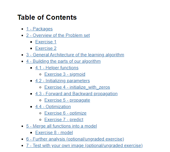
1 - Packages

First, let’s run the cell below to import all the packages that you will need during this assignment.

• numpy is the fundamental package for scientific computing with Python.
• h5py is a common package to interact with a dataset that is stored on an H5 file.
• matplotlib is a famous library to plot graphs in Python.
• PIL and scipy are used here to test your model with your own picture at the end.

import numpy as np
import copy
import matplotlib.pyplot as plt
import h5py
import scipy
from PIL import Image
from scipy import ndimage
from lr_utils import load_dataset
from public_tests import *

%matplotlib inline
%load_ext autoreload
%autoreload 2

2 - Overview of the Problem set

Problem Statement: You are given a dataset (“data.h5”) containing:
- a training set of m_train images labeled as cat (y=1) or non-cat (y=0)
- a test set of m_test images labeled as cat or non-cat
- each image is of shape (num_px, num_px, 3) where 3 is for the 3 channels (RGB). Thus, each image is square (height = num_px) and (width = num_px).

You will build a simple image-recognition algorithm that can correctly classify pictures as cat or non-cat.

Let’s get more familiar with the dataset. Load the data by running the following code.

# Loading the data (cat/non-cat)
train_set_x_orig, train_set_y, test_set_x_orig, test_set_y, classes = load_dataset()

We added “_orig” at the end of image datasets (train and test) because we are going to preprocess them. After preprocessing, we will end up with train_set_x and test_set_x (the labels train_set_y and test_set_y don’t need any preprocessing).

Each line of your train_set_x_orig and test_set_x_orig is an array representing an image. You can visualize an example by running the following code. Feel free also to change the index value and re-run to see other images.

# Example of a picture
index = 25
plt.imshow(train_set_x_orig[index])
print ("y = " + str(train_set_y[:, index]) + ", it's a '" + classes[np.squeeze(train_set_y[:, index])].decode("utf-8") +  "' picture.")

Output

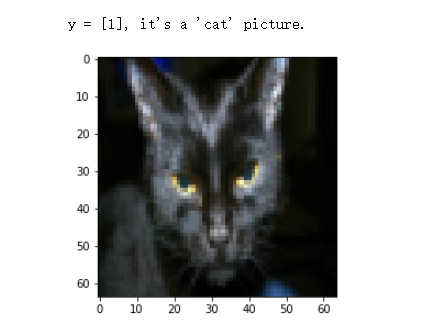
Many software bugs in deep learning come from having matrix/vector dimensions that don’t fit. If you can keep your matrix/vector dimensions straight you will go a long way toward eliminating many bugs.

Exercise 1

Find the values for:

• m_train (number of training examples)
• m_test (number of test examples)
• num_px (= height = width of a training image)
  Remember that train_set_x_orig is a numpy-array of shape (m_train, num_px, num_px, 3). For instance, you can access m_train by writing train_set_x_orig.shape[0].

#(≈ 3 lines of code)
# m_train = 
# m_test = 
# num_px = 
# YOUR CODE STARTS HERE
m_train = train_set_x_orig.shape[0]
m_test = test_set_x_orig.shape[0]
num_px = train_set_x_orig[0].shape[0]

# YOUR CODE ENDS HERE

print ("Number of training examples: m_train = " + str(m_train))
print ("Number of testing examples: m_test = " + str(m_test))
print ("Height/Width of each image: num_px = " + str(num_px))
print ("Each image is of size: (" + str(num_px) + ", " + str(num_px) + ", 3)")
print ("train_set_x shape: " + str(train_set_x_orig.shape))
print ("train_set_y shape: " + str(train_set_y.shape))
print ("test_set_x shape: " + str(test_set_x_orig.shape))
print ("test_set_y shape: " + str(test_set_y.shape))

Output

Number of training examples: m_train = 209
Number of testing examples: m_test = 50
Height/Width of each image: num_px = 64
Each image is of size: (64, 64, 3)
train_set_x shape: (209, 64, 64, 3)
train_set_y shape: (1, 209)
test_set_x shape: (50, 64, 64, 3)
test_set_y shape: (1, 50)

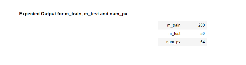
For convenience, you should now reshape images of shape (num_px, num_px, 3) in a numpy-array of shape (num_px $\ast$ num_px $\ast$ 3, 1). After this, our training (and test) dataset is a numpy-array where each column represents a flattened image. There should be m_train (respectively m_test) columns.

Exercise 2

Reshape the training and test data sets so that images of size (num_px, num_px, 3) are flattened into single vectors of shape (num_px $\ast$ num_px $\ast$ 3, 1).

A trick when you want to flatten a matrix X of shape (a,b,c,d) to a matrix X_flatten of shape (b$\ast$c$\ast$d, a) is to use:

X_flatten = X.reshape(X.shape[0], -1).T      # X.T is the transpose of X

# Reshape the training and test examples
#(≈ 2 lines of code)
# train_set_x_flatten = ...
# test_set_x_flatten = ...
# YOUR CODE STARTS HERE
train_set_x_flatten = train_set_x_orig.reshape(train_set_x_orig.shape[0], -1).T
test_set_x_flatten = test_set_x_orig.reshape(test_set_x_orig.shape[0], -1).T

# YOUR CODE ENDS HERE

# Check that the first 10 pixels of the second image are in the correct place
assert np.alltrue(train_set_x_flatten[0:10, 1] == [196, 192, 190, 193, 186, 182, 188, 179, 174, 213]), "Wrong solution. Use (X.shape[0], -1).T."
assert np.alltrue(test_set_x_flatten[0:10, 1] == [115, 110, 111, 137, 129, 129, 155, 146, 145, 159]), "Wrong solution. Use (X.shape[0], -1).T."

print ("train_set_x_flatten shape: " + str(train_set_x_flatten.shape))
print ("train_set_y shape: " + str(train_set_y.shape))
print ("test_set_x_flatten shape: " + str(test_set_x_flatten.shape))
print ("test_set_y shape: " + str(test_set_y.shape))

Output

train_set_x_flatten shape: (12288, 209)
train_set_y shape: (1, 209)
test_set_x_flatten shape: (12288, 50)
test_set_y shape: (1, 50)

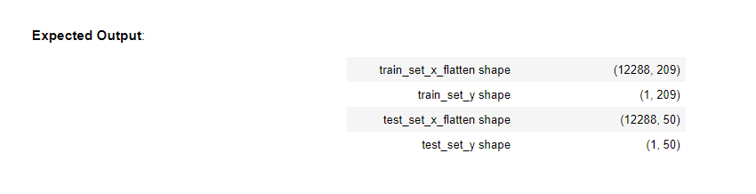
To represent color images, the red, green and blue channels (RGB) must be specified for each pixel, and so the pixel value is actually a vector of three numbers ranging from 0 to 255.

One common preprocessing step in machine learning is to center and standardize your dataset, meaning that you substract the mean of the whole numpy array from each example, and then divide each example by the standard deviation of the whole numpy array. But for picture datasets, it is simpler and more convenient and works almost as well to just divide every row of the dataset by 255 (the maximum value of a pixel channel).

Let’s standardize our dataset.

train_set_x = train_set_x_flatten / 255.
test_set_x = test_set_x_flatten / 255.

3 - General Architecture of the learning algorithm

It’s time to design a simple algorithm to distinguish cat images from non-cat images.

You will build a Logistic Regression, using a Neural Network mindset. The following Figure explains why Logistic Regression is actually a very simple Neural Network!

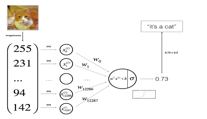
Mathematical expression of the algorithm:

For one example $x^{(i)}$:
$$z^{(i)}=w^T{x}^{(i)}+b\text{\hspace{1em}(1)}$$
$${\hat{y}}^{(i)}=a^{(i)}=sigmoid(z^{(i)})\text{\hspace{1em}(2)}$$
$$\mathcal{L}(a^{(i)},y^{(i)})=-y^{(i)}\log (a^{(i)})-(1-y^{(i)})\log (1-a^{(i)})\text{\hspace{1em}(3)}$$

The cost is then computed by summing over all training examples:
$$J=\frac{1}{m}\sum _{i=1}^m\mathcal{L}(a^{(i)},y^{(i)})\text{\hspace{1em}(6)}$$

Key steps:
In this exercise, you will carry out the following steps:

• Initialize the parameters of the model
• Learn the parameters for the model by minimizing the cost
• Use the learned parameters to make predictions (on the test set)
• Analyse the results and conclude

4 - Building the parts of our algorithm

The main steps for building a Neural Network are:

1. Define the model structure (such as number of input features)
2. Initialize the model’s parameters
3. Loop:
   • Calculate current loss (forward propagation)
   • Calculate current gradient (backward propagation)
   • Update parameters (gradient descent)

You often build 1-3 separately and integrate them into one function we call model().

4.1 - Helper functions

Exercise 3 - sigmoid

Using your code from “Python Basics”, implement sigmoid(). As you’ve seen in the figure above, you need to compute $sigmoid(z)=\frac{1}{1+e^{-z}}$ for $z=w^{T}x+b$ to make predictions. Use np.exp().

# GRADED FUNCTION: sigmoid

def sigmoid(z):
    """
    Compute the sigmoid of z

    Arguments:
    z -- A scalar or numpy array of any size.

    Return:
    s -- sigmoid(z)
    """

    #(≈ 1 line of code)
    # s = ...
    # YOUR CODE STARTS HERE
    s = 1 / (1 + np.exp(-z))
    
    # YOUR CODE ENDS HERE
    
    return s

print ("sigmoid([0, 2]) = " + str(sigmoid(np.array([0,2]))))

sigmoid_test(sigmoid)

Output

sigmoid([0, 2]) = [0.5        0.88079708]
All tests passed!

x = np.array([0.5, 0, 2.0])
output = sigmoid(x)
print(output)

Output

[0.62245933 0.5        0.88079708]

4.2 - Initializing parameters

Exercise 4 - initialize_with_zeros

Implement parameter initialization in the cell below. You have to initialize w as a vector of zeros. If you don’t know what numpy function to use, look up np.zeros() in the Numpy library’s documentation.

# GRADED FUNCTION: initialize_with_zeros

def initialize_with_zeros(dim):
    """
    This function creates a vector of zeros of shape (dim, 1) for w and initializes b to 0.
    
    Argument:
    dim -- size of the w vector we want (or number of parameters in this case)
    
    Returns:
    w -- initialized vector of shape (dim, 1)
    b -- initialized scalar (corresponds to the bias) of type float
    """
    
    # (≈ 2 lines of code)
    # w = ...
    # b = ...
    # YOUR CODE STARTS HERE
    w = np.zeros((dim, 1))
    b = 0.0
    
    # YOUR CODE ENDS HERE

    return w, b

dim = 2
w, b = initialize_with_zeros(dim)

assert type(b) == float
print ("w = " + str(w))
print ("b = " + str(b))

initialize_with_zeros_test_1(initialize_with_zeros)
initialize_with_zeros_test_2(initialize_with_zeros)

Output

w = [[0.]
 [0.]]
b = 0.0
First test passed!
Second test passed!

4.3 - Forward and Backward propagation

Now that your parameters are initialized, you can do the “forward” and “backward” propagation steps for learning the parameters.

Exercise 5 - propagate

Implement a function propagate() that computes the cost function and its gradient.

Hints:

Forward Propagation:

• You get X
• You compute $A=\sigma (w^{T}X+b)=(a^{(1)},a^{(2)},...,a^{(m-1)},a^{(m)})$
• You calculate the cost function: $J=-\frac{1}{m}{\sum }_{i=1}^m(y^{(i)}\log (a^{(i)})+(1-y^{(i)})\log (1-a^{(i)}))$

Here are the two formulas you will be using:

$$\frac{\partial J}{\partial w}=\frac{1}{m}X(A-Y{)}^T\text{\hspace{1em}(7)}$$
$$\frac{\partial J}{\partial b}=\frac{1}{m}\sum _{i=1}^m(a^{(i)}-y^{(i)})\text{\hspace{1em}(8)}$$

# GRADED FUNCTION: propagate

def propagate(w, b, X, Y):
    """
    Implement the cost function and its gradient for the propagation explained above

    Arguments:
    w -- weights, a numpy array of size (num_px * num_px * 3, 1)
    b -- bias, a scalar
    X -- data of size (num_px * num_px * 3, number of examples)
    Y -- true "label" vector (containing 0 if non-cat, 1 if cat) of size (1, number of examples)

    Return:
    grads -- dictionary containing the gradients of the weights and bias
            (dw -- gradient of the loss with respect to w, thus same shape as w)
            (db -- gradient of the loss with respect to b, thus same shape as b)
    cost -- negative log-likelihood cost for logistic regression
    
    Tips:
    - Write your code step by step for the propagation. np.log(), np.dot()
    """
    
    m = X.shape[1]
    
    # FORWARD PROPAGATION (FROM X TO COST)
    #(≈ 2 lines of code)
    # compute activation
    # A = ...
    # compute cost by using np.dot to perform multiplication. 
    # And don't use loops for the sum.
    # cost = ...                                
    # YOUR CODE STARTS HERE
    A = sigmoid(np.dot(w.T, X) + b)
    cost = - 1 / m * np.sum(Y * np.log(A) + (1 - Y) * np.log(1 - A))
    
    # YOUR CODE ENDS HERE

    # BACKWARD PROPAGATION (TO FIND GRAD)
    #(≈ 2 lines of code)
    # dw = ...
    # db = ...
    # YOUR CODE STARTS HERE
    dw = 1 / m * np.dot(X, (A - Y).T)
    db = 1 / m * np.sum(A - Y)
    
    # YOUR CODE ENDS HERE
    cost = np.squeeze(np.array(cost))

    
    grads = {"dw": dw,
             "db": db}
    
    return grads, cost

w =  np.array([[1.], [2]])
b = 1.5

# X is using 3 examples, with 2 features each
# Each example is stacked column-wise
X = np.array([[1., -2., -1.], [3., 0.5, -3.2]])
Y = np.array([[1, 1, 0]])
grads, cost = propagate(w, b, X, Y)

assert type(grads["dw"]) == np.ndarray
assert grads["dw"].shape == (2, 1)
assert type(grads["db"]) == np.float64


print ("dw = " + str(grads["dw"]))
print ("db = " + str(grads["db"]))
print ("cost = " + str(cost))

propagate_test(propagate)

Output

dw = [[ 0.25071532]
 [-0.06604096]]
db = -0.1250040450043965
cost = 0.15900537707692405
All tests passed!

Expected output

dw = [[ 0.25071532]
 [-0.06604096]]
db = -0.1250040450043965
cost = 0.15900537707692405

4.4 - Optimization

• You have initialized your parameters.
• You are also able to compute a cost function and its gradient.
• Now, you want to update the parameters using gradient descent.

Exercise 6 - optimize

Write down the optimization function. The goal is to learn $w$ and $b$ by minimizing the cost function $J$. For a parameter $\theta$, the update rule is $\theta =\theta -\alpha d\theta$, where $\alpha$ is the learning rate.

# GRADED FUNCTION: optimize

def optimize(w, b, X, Y, num_iterations=100, learning_rate=0.009, print_cost=False):
    """
    This function optimizes w and b by running a gradient descent algorithm
    
    Arguments:
    w -- weights, a numpy array of size (num_px * num_px * 3, 1)
    b -- bias, a scalar
    X -- data of shape (num_px * num_px * 3, number of examples)
    Y -- true "label" vector (containing 0 if non-cat, 1 if cat), of shape (1, number of examples)
    num_iterations -- number of iterations of the optimization loop
    learning_rate -- learning rate of the gradient descent update rule
    print_cost -- True to print the loss every 100 steps
    
    Returns:
    params -- dictionary containing the weights w and bias b
    grads -- dictionary containing the gradients of the weights and bias with respect to the cost function
    costs -- list of all the costs computed during the optimization, this will be used to plot the learning curve.
    
    Tips:
    You basically need to write down two steps and iterate through them:
        1) Calculate the cost and the gradient for the current parameters. Use propagate().
        2) Update the parameters using gradient descent rule for w and b.
    """
    
    w = copy.deepcopy(w)
    b = copy.deepcopy(b)
    
    costs = []
    
    for i in range(num_iterations):
        # (≈ 1 lines of code)
        # Cost and gradient calculation 
        # grads, cost = ...
        # YOUR CODE STARTS HERE
        grads, cost = propagate(w, b, X, Y)
        
        # YOUR CODE ENDS HERE
        
        # Retrieve derivatives from grads
        dw = grads["dw"]
        db = grads["db"]
        
        # update rule (≈ 2 lines of code)
        # w = ...
        # b = ...
        # YOUR CODE STARTS HERE
        w = w - learning_rate * dw
        b = b - learning_rate * db
        
        # YOUR CODE ENDS HERE
        
        # Record the costs
        if i % 100 == 0:
            costs.append(cost)
        
            # Print the cost every 100 training iterations
            if print_cost:
                print ("Cost after iteration %i: %f" %(i, cost))
    
    params = {"w": w,
              "b": b}
    
    grads = {"dw": dw,
             "db": db}
    
    return params, grads, costs

params, grads, costs = optimize(w, b, X, Y, num_iterations=100, learning_rate=0.009, print_cost=False)

print ("w = " + str(params["w"]))
print ("b = " + str(params["b"]))
print ("dw = " + str(grads["dw"]))
print ("db = " + str(grads["db"]))
print("Costs = " + str(costs))

optimize_test(optimize)

Output

w = [[0.80956046]
 [2.0508202 ]]
b = 1.5948713189708588
dw = [[ 0.17860505]
 [-0.04840656]]
db = -0.08888460336847771
Costs = [array(0.15900538)]
All tests passed!

Exercise 7 - predict

The previous function will output the learned w and b. We are able to use w and b to predict the labels for a dataset X. Implement the predict() function. There are two steps to computing predictions:

1. Calculate $\hat{Y}=A=\sigma (w^{T}X+b)$

2. Convert the entries of a into 0 (if activation <= 0.5) or 1 (if activation > 0.5), stores the predictions in a vector Y_prediction. If you wish, you can use an if/else statement in a for loop (though there is also a way to vectorize this).

# GRADED FUNCTION: predict

def predict(w, b, X):
    '''
    Predict whether the label is 0 or 1 using learned logistic regression parameters (w, b)
    
    Arguments:
    w -- weights, a numpy array of size (num_px * num_px * 3, 1)
    b -- bias, a scalar
    X -- data of size (num_px * num_px * 3, number of examples)
    
    Returns:
    Y_prediction -- a numpy array (vector) containing all predictions (0/1) for the examples in X
    '''
    
    m = X.shape[1]
    Y_prediction = np.zeros((1, m))
    w = w.reshape(X.shape[0], 1)
    
    # Compute vector "A" predicting the probabilities of a cat being present in the picture
    #(≈ 1 line of code)
    # A = ...
    # YOUR CODE STARTS HERE
    A = sigmoid(np.dot(w.T, X) + b)
    
    # YOUR CODE ENDS HERE
    
    for i in range(A.shape[1]):
        
        # Convert probabilities A[0,i] to actual predictions p[0,i]
        #(≈ 4 lines of code)
        # if A[0, i] > ____ :
        #     Y_prediction[0,i] = 
        # else:
        #     Y_prediction[0,i] = 
        # YOUR CODE STARTS HERE
        if A[0, i] > 0.5:
            Y_prediction[0, i] = 1
        else:
            Y_prediction[0, i] = 0
        
        # YOUR CODE ENDS HERE
    
    return Y_prediction

w = np.array([[0.1124579], [0.23106775]])
b = -0.3
X = np.array([[1., -1.1, -3.2],[1.2, 2., 0.1]])
print ("predictions = " + str(predict(w, b, X)))

predict_test(predict)

Output

predictions = [[1. 1. 0.]]
All tests passed!

What to remember:

You’ve implemented several functions that:

• Initialize (w,b)
• Optimize the loss iteratively to learn parameters (w,b):
  • Computing the cost and its gradient
  • Updating the parameters using gradient descent
• Use the learned (w,b) to predict the labels for a given set of examples

5 - Merge all functions into a model

You will now see how the overall model is structured by putting together all the building blocks (functions implemented in the previous parts) together, in the right order.

Exercise 8 - model

Implement the model function. Use the following notation:

• Y_prediction_test for your predictions on the test set
• Y_prediction_train for your predictions on the train set
• parameters, grads, costs for the outputs of optimize()

# GRADED FUNCTION: model

def model(X_train, Y_train, X_test, Y_test, num_iterations=2000, learning_rate=0.5, print_cost=False):
    """
    Builds the logistic regression model by calling the function you've implemented previously
    
    Arguments:
    X_train -- training set represented by a numpy array of shape (num_px * num_px * 3, m_train)
    Y_train -- training labels represented by a numpy array (vector) of shape (1, m_train)
    X_test -- test set represented by a numpy array of shape (num_px * num_px * 3, m_test)
    Y_test -- test labels represented by a numpy array (vector) of shape (1, m_test)
    num_iterations -- hyperparameter representing the number of iterations to optimize the parameters
    learning_rate -- hyperparameter representing the learning rate used in the update rule of optimize()
    print_cost -- Set to True to print the cost every 100 iterations
    
    Returns:
    d -- dictionary containing information about the model.
    """
    # (≈ 1 line of code)   
    # initialize parameters with zeros
    # and use the "shape" function to get the first dimension of X_train
    # w, b = ...
    
    #(≈ 1 line of code)
    # Gradient descent 
    # params, grads, costs = ...
    
    # Retrieve parameters w and b from dictionary "params"
    # w = ...
    # b = ...
    
    # Predict test/train set examples (≈ 2 lines of code)
    # Y_prediction_test = ...
    # Y_prediction_train = ...
    
    # YOUR CODE STARTS HERE
    w, b = initialize_with_zeros(X_train.shape[0])
    params, grads, costs = optimize(w, b, X_train, Y_train, num_iterations, learning_rate, print_cost)
    
    w = params["w"]
    b = params["b"]
    Y_prediction_test = predict(w, b, X_test) 
    Y_prediction_train = predict(w, b, X_train)
    
    
    # YOUR CODE ENDS HERE

    # Print train/test Errors
    if print_cost:
        print("train accuracy: {} %".format(100 - np.mean(np.abs(Y_prediction_train - Y_train)) * 100))
        print("test accuracy: {} %".format(100 - np.mean(np.abs(Y_prediction_test - Y_test)) * 100))

    
    d = {"costs": costs,
         "Y_prediction_test": Y_prediction_test, 
         "Y_prediction_train" : Y_prediction_train, 
         "w" : w, 
         "b" : b,
         "learning_rate" : learning_rate,
         "num_iterations": num_iterations}
    
    return d

from public_tests import *

model_test(model)

Output

All tests passed!

If you pass all the tests, run the following cell to train your model.

logistic_regression_model = model(train_set_x, train_set_y, test_set_x, test_set_y, num_iterations=2000, learning_rate=0.005, print_cost=True)

Output

Cost after iteration 0: 0.693147
Cost after iteration 100: 0.584508
Cost after iteration 200: 0.466949
Cost after iteration 300: 0.376007
Cost after iteration 400: 0.331463
Cost after iteration 500: 0.303273
Cost after iteration 600: 0.279880
Cost after iteration 700: 0.260042
Cost after iteration 800: 0.242941
Cost after iteration 900: 0.228004
Cost after iteration 1000: 0.214820
Cost after iteration 1100: 0.203078
Cost after iteration 1200: 0.192544
Cost after iteration 1300: 0.183033
Cost after iteration 1400: 0.174399
Cost after iteration 1500: 0.166521
Cost after iteration 1600: 0.159305
Cost after iteration 1700: 0.152667
Cost after iteration 1800: 0.146542
Cost after iteration 1900: 0.140872
train accuracy: 99.04306220095694 %
test accuracy: 70.0 %

Comment: Training accuracy is close to 100%. This is a good sanity check: your model is working and has high enough capacity to fit the training data. Test accuracy is 70%. It is actually not bad for this simple model, given the small dataset we used and that logistic regression is a linear classifier. But no worries, you’ll build an even better classifier next week!

Also, you see that the model is clearly overfitting the training data. Later in this specialization you will learn how to reduce overfitting, for example by using regularization. Using the code below (and changing the index variable) you can look at predictions on pictures of the test set.

# Example of a picture that was wrongly classified.
index = 1
plt.imshow(test_set_x[:, index].reshape((num_px, num_px, 3)))
print ("y = " + str(test_set_y[0,index]) + ", you predicted that it is a \"" + classes[int(logistic_regression_model['Y_prediction_test'][0,index])].decode("utf-8") +  "\" picture.")

Output

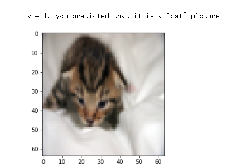
Let’s also plot the cost function and the gradients.

# Plot learning curve (with costs)
costs = np.squeeze(logistic_regression_model['costs'])
plt.plot(costs)
plt.ylabel('cost')
plt.xlabel('iterations (per hundreds)')
plt.title("Learning rate =" + str(logistic_regression_model["learning_rate"]))
plt.show()

Output

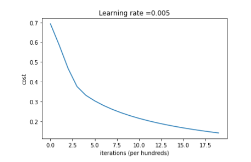
Interpretation:
You can see the cost decreasing. It shows that the parameters are being learned. However, you see that you could train the model even more on the training set. Try to increase the number of iterations in the cell above and rerun the cells. You might see that the training set accuracy goes up, but the test set accuracy goes down. This is called overfitting.

6 - Further analysis (optional/ungraded exercise)

Congratulations on building your first image classification model. Let’s analyze it further, and examine possible choices for the learning rate $\alpha$.

Choice of learning rate

Reminder:
In order for Gradient Descent to work you must choose the learning rate wisely. The learning rate $\alpha$ determines how rapidly we update the parameters. If the learning rate is too large we may “overshoot” the optimal value. Similarly, if it is too small we will need too many iterations to converge to the best values. That’s why it is crucial to use a well-tuned learning rate.

Let’s compare the learning curve of our model with several choices of learning rates. Run the cell below. This should take about 1 minute. Feel free also to try different values than the three we have initialized the learning_rates variable to contain, and see what happens.

learning_rates = [0.01, 0.001, 0.0001]
models = {}

for lr in learning_rates:
    print ("Training a model with learning rate: " + str(lr))
    models[str(lr)] = model(train_set_x, train_set_y, test_set_x, test_set_y, num_iterations=1500, learning_rate=lr, print_cost=False)
    print ('\n' + "-------------------------------------------------------" + '\n')

for lr in learning_rates:
    plt.plot(np.squeeze(models[str(lr)]["costs"]), label=str(models[str(lr)]["learning_rate"]))

plt.ylabel('cost')
plt.xlabel('iterations (hundreds)')

legend = plt.legend(loc='upper center', shadow=True)
frame = legend.get_frame()
frame.set_facecolor('0.90')
plt.show()

Output

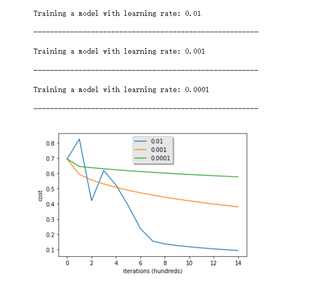
Interpretation:

• Different learning rates give different costs and thus different predictions results.
• If the learning rate is too large (0.01), the cost may oscillate up and down. It may even diverge (though in this example, using 0.01 still eventually ends up at a good value for the cost).
• A lower cost doesn’t mean a better model. You have to check if there is possibly overfitting. It happens when the training accuracy is a lot higher than the test accuracy.
• In deep learning, we usually recommend that you:
  • Choose the learning rate that better minimizes the cost function.
  • If your model overfits, use other techniques to reduce overfitting. (We’ll talk about this in later videos.)

7 - Test with your own image (optional/ungraded exercise)

Congratulations on finishing this assignment. You can use your own image and see the output of your model. To do that:
1. Click on “File” in the upper bar of this notebook, then click “Open” to go on your Coursera Hub.
2. Add your image to this Jupyter Notebook’s directory, in the “images” folder
3. Change your image’s name in the following code
4. Run the code and check if the algorithm is right (1 = cat, 0 = non-cat)!

# change this to the name of your image file
my_image = "my_image.jpg"   

# We preprocess the image to fit your algorithm.
fname = "images/" + my_image
image = np.array(Image.open(fname).resize((num_px, num_px)))
plt.imshow(image)
image = image / 255.
image = image.reshape((1, num_px * num_px * 3)).T
my_predicted_image = predict(logistic_regression_model["w"], logistic_regression_model["b"], image)

print("y = " + str(np.squeeze(my_predicted_image)) + ", your algorithm predicts a \"" + classes[int(np.squeeze(my_predicted_image)),].decode("utf-8") +  "\" picture.")

Output

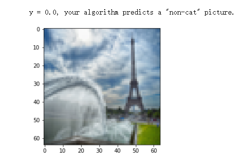
What to remember from this assignment:

1. Preprocessing the dataset is important.
2. You implemented each function separately: initialize(), propagate(), optimize(). Then you built a model().
3. Tuning the learning rate (which is an example of a “hyperparameter”) can make a big difference to the algorithm. You will see more examples of this later in this course!

Finally, if you’d like, we invite you to try different things on this Notebook. Make sure you submit before trying anything. Once you submit, things you can play with include:

• Play with the learning rate and the number of iterations
• Try different initialization methods and compare the results
• Test other preprocessings (center the data, or divide each row by its standard deviation)

Grades

其他

Commit template

git commit -m "Finish Week 02 of Neural Networks and Deep Learning"

英文发音

下面的英语是2022年7月做的笔记，当时零基础入门深度学习，还是在Coursera上直接听的英文课程，学的有点吃力。

不同不要再用different啦，用distinct

Computing this function actually has three distinct steps. 计算这个函数有三个不同的步骤

We’ll go through an example.我们会看一个例子

在后面几张幻灯片中可以看到: in the next couple of slides

we’ll see in the next couple of slides

看下一个视频：

Let’s go into the next video.进入到下一个视频

Let’s go on to the next video.

如何你去看微积分的书: if you go to calculus textbook

So if you go to calculus textbook, you find that when you take the
derivative of log(a).

on the previous slide: 在上一页幻灯片上

Let’s nudge a slightly to the right：稍微右移一点

has a ratio of xxx to xxx: 有什么样的占比

One way to see that is that, wherever you draw this little triangle. The height, divided by the width, always has a ratio of three to one.

infinitesimal 英 [ˌɪnfɪnɪˈtesɪml]：无穷小，无限小；极小的，微量的

nudge 英 [nʌdʒ] ： 渐渐推开，达到，接近

foray 英 [ˈfɒreɪ]：(改变职业、活动的)尝试;

in the foray into xxx: 在深入学习xxx的过程中

Open up the box: 打开盒子

peer a little bit further into the details of xxx: 瞥见更细节的一些东西

翻译：但我认为，在本周深入学习的过程中，我们应该打开盒子，深入研究微积分的细节。

But I thought that in this foray into deep learning that this week, we should open up the box and peer a little bit further into the details of calculus.

this quantity: 中文数学中的这个量，那个量，比如a这个量

confusing to somebody: 对xx来说有点不好理解

That is a bit confusing to some people

colon equals to: 冒号等于 :=

Going to use colon equals
to represent updating w.

strip parenthesis: 大括号，带括号

use this notational convention: 符号上的规范

Some new and interesting ideas one can pick up: 可以学习到的很多有趣的新颖的ideas

I think that there’ll be some new and interesting ideas for you to pick up in this week’s materials.

remarkably: rəˈmärkəblē 显著地

---

2024年5月1日做的英文笔记：无

后记

2024年5月10日11点20分完成week 2的学习。