Natural Language Processing with Attention Models
Course Certificate

本文是学习这门课 Natural Language Processing with Attention Models的学习笔记,如有侵权,请联系删除。
文章目录
- Natural Language Processing with Attention Models
- Week 01: Neural Machine Translation
-
- Seq2seq
- Seq2seq Model with Attention
- Ungraded Lab: Basic Attention
- Background on seq2seq
- Queries, Keys, Values, and Attention
- Ungraded Lab: Scaled Dot-Product Attention
- Setup for Machine Translation
- Teacher Forcing
- NMT Model with Attention
- BLEU Score
- Ungraded Lab: BLEU Score
- ROUGE-N Score
- Sampling and Decoding
- Beam Search
- Minimum Bayes Risk
- Quiz
- Programming Assignment: NMT with Attention (Tensorflow)
-
- 1. Data Preparation
- 2. NMT model with attention
- Exercise 1 - Encoder
- Exercise 2 - CrossAttention
- Exercise 3 - Decoder
- Exercise 4 - Translator
- 3. Training
- 4. Using the model for inference
- Exercise 5 - translate
- 5. Minimum Bayes-Risk Decoding
- Comparing overlaps
- Exercise 6 - rouge1_similarity
- Computing the Overall Score
- Exercise 7 - average_overlap
- mbr_decode
- Grades
- 后记
Week 01: Neural Machine Translation
Discover some of the shortcomings of a traditional seq2seq model and how to solve for them by adding an attention mechanism, then build a Neural Machine Translation model with Attention that translates English sentences into German.
Learning Objectives
- Explain how an Encoder/Decoder model works
- Apply word alignment for machine translation
- Train a Neural Machine Translation model with Attention
- Develop intuition for how teacher forcing helps a translation model check its predictions
- Use BLEU score and ROUGE score to evaluate machine-generated text quality
- Describe several decoding methods including MBR and Beam search
Seq2seq
Good to see you again. You will now learn about
neural machine translation, and you’ll see what
the architecture of this neural
network looks like. You will also learn which words the neural network
is focusing on when translating from
one language to another. Let’s formalize this task. To get started on
this week’s material, I’ll introduce you to neural machine
translation along with the model that was traditionally used for its implementation. The seq2seq model. Then, I’ll talk about some
of this models shortcomings and the solution as they
lead into the model that you’ll be using in
this week’s assignments. Exciting stuff. Let’s go.
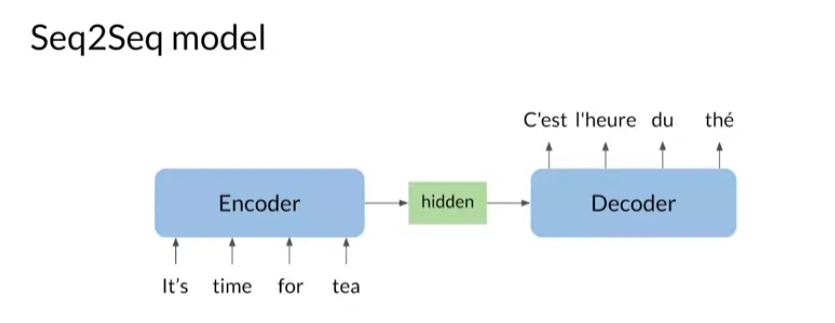
In neural machine translation, you’re using an
encoder and a decoder to translate from one
language to another. For example, you
could translate, it’s time for tea from English to French, C’est l’heure du the. To do this, you could use a
machine translation system that has LSTMs for both
encoding and decoding. The traditional seq2seq
model was introduced by Google in 2014 and it was a revelation
at the time. Basically, it works by
taking one sequence of items such as words and its
output, another sequence. The way this is
done is by mapping variable length sequences
to a fixed length memory, which in machine translation, encodes the overall
meaning of sentences.
For example, you can have a text of length that varies and you can encode
it into a vector or fixed dimension
like 300, for example. This feature is what’s made this model a powerhouse
for machine translation. Additionally, the
inputs and outputs don’t need to have
matching lengths, which is a desirable feature
when translating texts. Then you might recall the
vanishing and exploding gradients problems from
earlier in the specialization. In seq2seq model, LSTMs and GRUs are typically
used to avoid these problems. As I mentioned, in
a seq2seq model, you have an encoder
and a decoder.
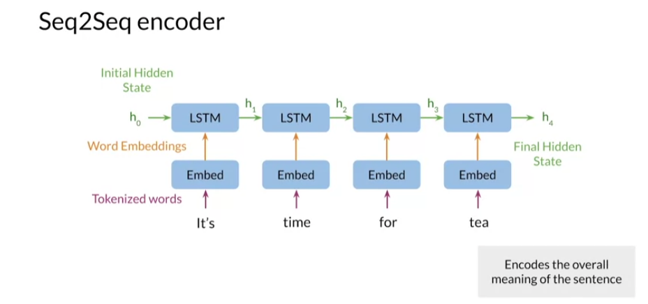
The encoder takes
word tokens as input, and it returns its final
hidden states as outputs. This hidden state is
used by the decoder to generate the translated sentence
in the target language. Before moving on, let’s look closer at the
encoder and decoder. The encoder typically consists
of an embedding layer and an LSTM module with
one or more layers. The embedding layer
transforms words tokenized first into a vector for
input to the LSTM module. At each step in the
input sequence, the LSTM module receives inputs
from the embedding layer, as well as the hidden states
from the previous step. The encoder returns the hidden
states of the final step, shown here as h_4. This final hidden
state has information from the whole sentence and it encodes its
overall meaning.
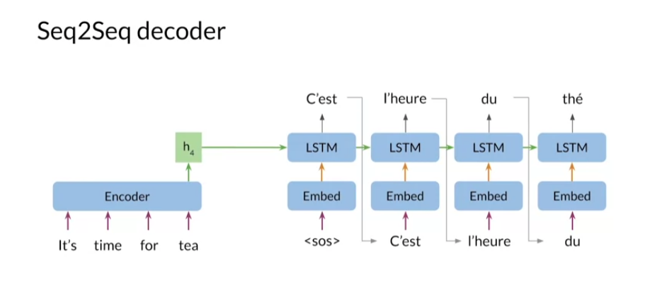
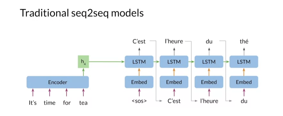
The decoder is constructed similarly with an embedding
layer and an LSTM layer. You use the output
word of a step as the input word
for the next step. You also pass the LSTM hidden
state to the next step. You start the input sequence where there is start of sequence token denoted as SOS here. The first step, C’est, as the most probable next word. Then you use C’est as the
input word for the next step and repeat to generate the rest of the sentence
l’heure du the.
One major limitation of the
traditional seq2seq model is what’s referred to as
the information bottleneck. Since seq2seq uses a
fixed length memory for the hidden states, long sequences
become problematic. This is due to the fact that in traditional
seq2seq models, only a fixed amount of
information can be passed from the encoder to
the decoder no matter how much information is
contained in the input sequence. The power of seq2seq, which allows for inputs and outputs to be different sizes, becomes not effective when
the input sequence is long. The result is lower
model performance, a sequence size increases
and that’s no good.


The issue with having one fixed size encoder hidden states is that it struggles to compress longer sequences and it
ends up throttling itself and punishing the decoder who only wants to make
a good prediction. One workaround is to use
the encoder hidden states for each word instead of trying to smash it all into
one big vector. But this model would have flaws
with memory and contexts. How could you build a time
and memory efficient model that predicts accurately
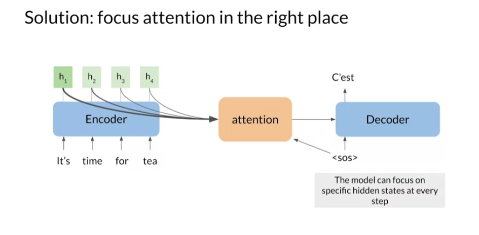
from a long sequence? This becomes possible if the
model has a way to select and focus on the most important
words at each time step. You can think of this as giving the model a new layer to
process this information, which in the slide
is called attention. If you provide the information specific to each input word, you can give the
model a way to focus it’s attention in
the right place at each step of the
decoding process. That is good progress.
Up next, you’ll get
a conceptual idea of what this new layer
is doing and why. You now have an overview of
neural machine translation, and you have a rough idea of what attention
is looking like. You know which words the
model is focusing on when translating from one
language to another language.
Seq2Seq是一种序列到序列的模型,通常用于自然语言处理任务,比如机器翻译和文本摘要。它由两个主要部分组成:编码器(encoder)和解码器(decoder)。
编码器(Encoder):接受输入序列,并将其转换为隐藏状态向量。编码器通常使用循环神经网络(RNN)或者变种(比如长短时记忆网络(LSTM)或门控循环单元(GRU))来处理输入序列,并捕捉输入序列中的信息。
解码器(Decoder):接受编码器生成的隐藏状态向量,并利用该向量生成输出序列。解码器也通常是一个循环神经网络,它会根据输入的隐藏状态和先前生成的标记来预测下一个标记。在训练期间,解码器通过将正确的目标标记传递给下一个时间步来生成序列。在推理阶段,解码器根据前一个时间步生成的标记来生成下一个标记,直到生成特殊的终止标记或达到最大输出长度。
Seq2Seq模型已经被广泛用于许多任务,它的灵活性和强大性使得它成为了自然语言处理领域的一个重要工具。
Seq2seq Model with Attention
Welcome. Attention is a
very important concepts and allows you to focus
where the model is looking at whenever
making a prediction. For example, when translating one paragraph from
English to French, you can focus on translating one sentence at a
time or even more, a couple of words at a time. Let’s dive into this concept. What we call attention
now was introduced in a landmark paper from
Dzmitry Bahdanau, KyungHyun Cho, and
Yoshua Bengio. The authors developed a method to fix the seq to seq models, and ability to translate
longer sentences. As you can see, attention was originally developed for
machine translation, but it’s since being used in many other domains
with great success. Before we move forward, I want to skip ahead
a bit and show you how well attention works. It’s surprising.
https://arxiv.org/abs/1409.0473
Title: Neural Machine Translation by Jointly Learning to Align and Translate
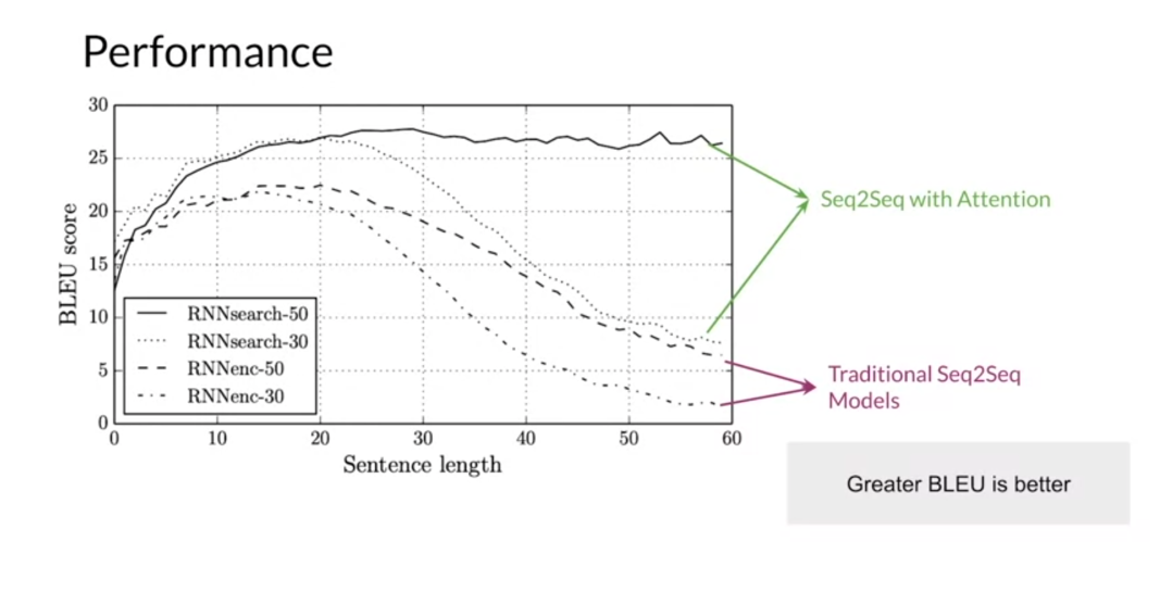
Here’s a comparison of
the performance between different models from
the Bahdanau paper using the bleu score, a performance metric that
you’ll learn about later. In brief, higher
scores are better, indicating more
correct translations. The dashed lines, they showed the scores for
bidirectional seq to seq model as the length of the input
sentence is increased. The 30 and 50 denotes the maximum sequence length
used to train the models. As you can see, the seq to seq models perform welfare sentences with
about 10-20 words, but they fall off beyond that. This is what you should expect. A seq to seq models
must store the meaning of the entire input sequence,
any single vector. The models developed
in this paper, RNN search 13-15, use bidirectional encoders and decoders, but with attention. First, these models
perform better than the traditional seqto seqmodels across all
sentence length. The RNN search 50 model has basically no fall off in performance as sentence
lengths increase. As you will see, this is because the models are able to focus on specific inputs to predict words in the output translation, instead of having to memorize
the entire input sentence.
Now I’ll show you the motivation behind attention
and how it works. Traditional seq to seq models, use the final hidden states of the encoder as the initial
hidden state of the decoder. This forces the encoder
to store the meaning of the entire input sequence
into this one hidden states.
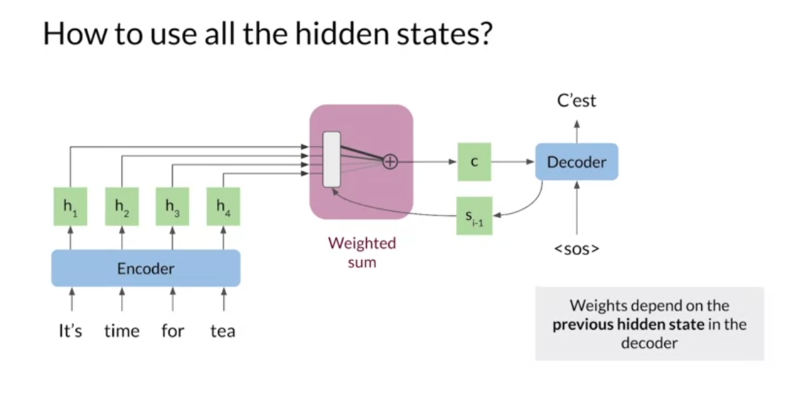
Instead of using only
the final hidden states, you can pass all the hidden
states to the decoder. However, this quickly
becomes inefficient as you must retain the
hidden states for each input step in memory. To solve this, you can combine the hidden
states into one vector, typically called
the context vector. The samples operation here
is the point-wise addition. Since the hidden vectors
are all the same size, you can just add up
these vector elements by elements to produce another
vector of the same size. But now the decoder is getting information
about each step. But It really only
needs information from the first few inputs steps to predict the first word. This isn’t that much
different from using the last hidden states
from LSTM or GRU.

The solution here is to wait certain encoder vectors more than others before the
point-wise addition, [inaudible] are
more important for the next decoder outputs
would have larger weights. That this way, the
context vector holds more information about the most important words and less information
about other words. But how are these
weights calculated to determine which input words
are important at each step? The decoders previous
hidden states, denoted as S i minus 1, contains information
about the previous words in the output translation. This means, you can compare
the decoder states with each encoder state to determine the most
important inputs. Intuitively, the decoder can
set the weights such that if it focuses on only the
most important inputs words for the next prediction, it decides which parts of the input sequence
to pay attention to.
Now step into the
attention layer to examine how the weights and context
vector are calculated. The goal of the attention
layer is to return a context vector that contains the relevant information
from the encoder states.
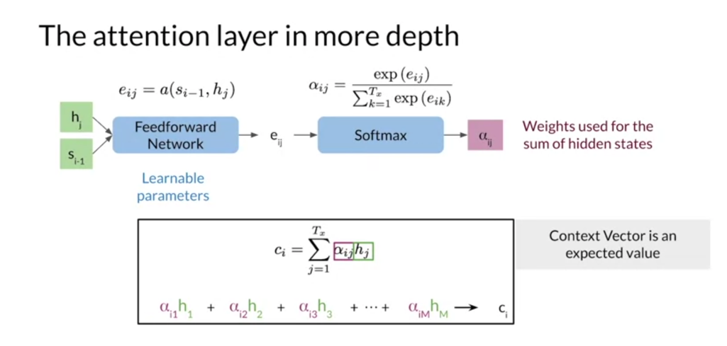
The first step is to
calculate the alignments, E_IJ, which is a
score of how well the inputs around J match
the expected output its I. The more the much, the higher of his score we will expect. This is done using the
feedforward neural network with the encoder and decoder
hidden states as inputs, where the weights for the
feedforward network are learned along with the rest
of the seq to seq model. The scores are then
turned into weights which range from zero to one
using the softmax function. This means the weights
can be thought of as a probability distribution
which sum to one.
Finally, each encoder
states is multiplied by its respective weights and sum together into one
context vector. Since the weights are the
probability distribution, this is equivalent
to calculating an expected value
across word alignments.
Next up, you’ll get a better understanding
of how all this works by implementing a simple version of the attention operation
from the Bahdanau paper. I have now shown
you how attention works and why it is important. In the next video, I will define what our keys, queries and values, and show you how to use
them in attention.
Seq2Seq模型的一个改进版本是带有注意力机制(Attention Mechanism)的Seq2Seq模型。在传统的Seq2Seq模型中,编码器将整个输入序列编码为一个固定长度的向量,然后解码器使用这个向量来生成输出序列。然而,这种固定长度的表示可能会丢失输入序列中重要的信息,特别是当输入序列很长时。
引入注意力机制可以解决这个问题。注意力机制允许解码器在生成每个输出标记时都可以“注意到”输入序列的不同部分,并根据需要分配不同的注意力权重。这样,解码器可以根据当前要生成的输出标记,动态地选择性地关注输入序列的不同部分,从而更好地捕捉输入序列中的重要信息。
具体来说,带有注意力机制的Seq2Seq模型包括以下几个关键组件:
编码器(Encoder):与传统的Seq2Seq模型相同,将输入序列编码为一系列隐藏状态向量。
解码器(Decoder):与传统的Seq2Seq模型相同,使用编码器最后的隐藏状态向量作为初始隐藏状态,并生成输出序列。
注意力机制(Attention Mechanism):在解码器的每个时间步,计算注意力权重,用于加权编码器的隐藏状态向量,以生成上下文向量。这个上下文向量会结合当前解码器的隐藏状态向量,用于生成当前时间步的输出。
带有注意力机制的Seq2Seq模型在处理长序列和捕捉序列中的局部依赖关系方面通常表现更好,因为它可以在生成每个输出标记时根据需要动态地关注输入序列的不同部分。这使得它成为许多序列到序列任务(如机器翻译、文本摘要等)中的首选模型之一。
Ungraded Lab: Basic Attention
Basic Attention Operation: Ungraded Lab
As you’ve learned, attention allows a seq2seq decoder to use information from each encoder step instead of just the final encoder hidden state. In the attention operation, the encoder outputs are weighted based on the decoder hidden state, then combined into one context vector. This vector is then used as input to the decoder to predict the next output step.
In this ungraded lab, you’ll implement a basic attention operation as described in Bhadanau, et al (2014) using Numpy.
This is a practice notebook, where you can train writing your code. All of the solutions are provided at the end of the notebook.
# Import the libraries and define the functions you will need for this lab
import numpy as np

def softmax(x, axis=0):
    """ Calculate softmax function for an array x along specified axis

        axis=0 calculates softmax across rows which means each column sums to 1
        axis=1 calculates softmax across columns which means each row sums to 1
    """
    return np.exp(x) / np.expand_dims(np.sum(np.exp(x), axis=axis), axis)
1: Calculating alignment scores
The first step is to calculate the alignment scores. This is a measure of similarity between the decoder hidden state and each encoder hidden state. From the paper, this operation looks like
e i j = v a ⊤ tanh ( W a s i − 1 + U a h j ) \large e_{ij} = v_a^\top \tanh{\left(W_a s_{i-1} + U_a h_j\right)} eij=va⊤tanh(Wasi−1+Uahj)
where W a ∈ R n × m W_a \in \mathbb{R}^{n\times m} Wa∈Rn×m, U a ∈ R n × m U_a \in \mathbb{R}^{n \times m} Ua∈Rn×m, and v a ∈ R m v_a \in \mathbb{R}^m va∈Rm
are the weight matrices and n n n is the hidden state size. In practice, this is implemented as a feedforward neural network with two layers, where m m m is the size of the layers in the alignment network. It looks something like:

Here h j h_j hj are the encoder hidden states for each input step j j j and s i − 1 s_{i - 1} si−1 is the decoder hidden state of the previous step. The first layer corresponds to W a W_a Wa and U a U_a Ua, while the second layer corresponds to v a v_a va.
To implement this, first concatenate the encoder and decoder hidden states to produce an array with size K × 2 n K \times 2n K×2n where K K K is the number of encoder states/steps. For this, use np.concatenate (docs). Note that there is only one decoder state so you’ll need to reshape it to successfully concatenate the arrays. The easiest way is to use decoder_state.repeat (docs) to match the hidden state array size.
Then, apply the first layer as a matrix multiplication between the weights and the concatenated input. Use the tanh function to get the activations. Finally, compute the matrix multiplication of the second layer weights and the activations. This returns the alignment scores.
hidden_size = 16
attention_size = 10
input_length = 5

np.random.seed(42)

# Synthetic vectors used to test
encoder_states = np.random.randn(input_length, hidden_size)
decoder_state = np.random.randn(1, hidden_size)

#print(decoder_state.repeat(input_length, axis=0))
# Weights for the neural network, these are typically learned through training
# Use these in the alignment function below as the layer weights
layer_1 = np.random.randn(2 * hidden_size, attention_size)
layer_2 = np.random.randn(attention_size, 1)

# Implement this function. Replace None with your code. Solution at the bottom of the notebook
def alignment(encoder_states, decoder_state):
    # First, concatenate the encoder states and the decoder state
    inputs = np.concatenate((encoder_states, decoder_state.repeat(input_length, axis=0)), axis=1)
    assert inputs.shape == (input_length, 2 * hidden_size)

    # Matrix multiplication of the concatenated inputs and layer_1, with tanh activation
    activations = np.tanh(np.dot(inputs, layer_1))
    assert activations.shape == (input_length, attention_size)

    # Matrix multiplication of the activations with layer_2. Remember that you don't need tanh here
    scores = np.dot(activations, layer_2)
    assert scores.shape == (input_length, 1)

    return scores
# Run this to test your alignment function
scores = alignment(encoder_states, decoder_state)
print(scores)
Output
[[4.35790943]
 [5.92373433]
 [4.18673175]
 [2.11437202]
 [0.95767155]]
If you implemented the function correctly, you should get these scores:
[[4.35790943]
 [5.92373433]
 [4.18673175]
 [2.11437202]
 [0.95767155]]
2: Turning alignment into weights
The next step is to calculate the weights from the alignment scores. These weights determine the encoder outputs that are the most important for the decoder output. These weights should be between 0 and 1. You can use the softmax function (which is already implemented above) to get these weights from the attention scores. Pass the attention scores vector to the softmax function to get the weights. Mathematically,
α i j = exp ( e i j ) ∑ k = 1 K exp ( e i k ) \large \alpha_{ij} = \frac{\exp{\left(e_{ij}\right)}}{\sum_{k=1}^K \exp{\left(e_{ik}\right)}} αij=∑k=1Kexp(eik)exp(eij)
3: Weight the encoder output vectors and sum
The weights tell you the importance of each input word with respect to the decoder state. In this step, you use the weights to modulate the magnitude of the encoder vectors. Words with little importance will be scaled down relative to important words. Multiply each encoder vector by its respective weight to get the alignment vectors, then sum up the weighted alignment vectors to get the context vector. Mathematically,
c i = ∑ j = 1 K α i j h j \large c_i = \sum_{j=1}^K\alpha_{ij} h_{j} ci=j=1∑Kαijhj
Implement these steps in the attention function below.
# Implement this function. Replace None with your code.
def attention(encoder_states, decoder_state):
    """ Example function that calculates attention, returns the context vector

        Arguments:
        encoder_vectors: NxM numpy array, where N is the number of vectors and M is the vector length
        decoder_vector: 1xM numpy array, M is the vector length, much be the same M as encoder_vectors
    """

    # First, calculate the alignment scores
    scores = alignment(encoder_states, decoder_state)

    # Then take the softmax of the alignment scores to get a weight distribution
    weights = softmax(scores) # 5x1

    # Multiply each encoder state by its respective weight
    weighted_scores = encoder_states * weights # 广播机制,逐元素相乘 5x16 vs. 5x1,后者变成5x16
    print(weighted_scores.shape)
    #print(weighted_scores)


    # Sum up weighted alignment vectors to get the context vector and return it
    context = np.sum(weighted_scores, axis=0)
    return context

context_vector = attention(encoder_states, decoder_state)
print(context_vector)
Output
(5, 16)
[-0.63514569  0.04917298 -0.43930867 -0.9268003   1.01903919 -0.43181409
  0.13365099 -0.84746874 -0.37572203  0.18279832 -0.90452701  0.17872958
 -0.58015282 -0.58294027 -0.75457577  1.32985756]
If you implemented the attention function correctly, the context vector should be
[-0.63514569  0.04917298 -0.43930867 -0.9268003   1.01903919 -0.43181409
  0.13365099 -0.84746874 -0.37572203  0.18279832 -0.90452701  0.17872958
 -0.58015282 -0.58294027 -0.75457577  1.32985756]
See below for solutions
# Solution
def alignment(encoder_states, decoder_state):
    # First, concatenate the encoder states and the decoder state.
    inputs = np.concatenate((encoder_states, decoder_state.repeat(input_length, axis=0)), axis=1)
    assert inputs.shape == (input_length, 2*hidden_size)

    # Matrix multiplication of the concatenated inputs and the first layer, with tanh activation
    activations = np.tanh(np.matmul(inputs, layer_1))
    assert activations.shape == (input_length, attention_size)

    # Matrix multiplication of the activations with the second layer. Remember that you don't need tanh here
    scores = np.matmul(activations, layer_2)
    assert scores.shape == (input_length, 1)

    return scores

# Run this to test your alignment function
scores = alignment(encoder_states, decoder_state)
print(scores)
# Solution
def attention(encoder_states, decoder_state):
    """ Example function that calculates attention, returns the context vector

        Arguments:
        encoder_vectors: NxM numpy array, where N is the number of vectors and M is the vector length
        decoder_vector: 1xM numpy array, M is the vector length, much be the same M as encoder_vectors
    """

    # First, calculate the dot product of each encoder vector with the decoder vector
    scores = alignment(encoder_states, decoder_state)

    # Then take the softmax of those scores to get a weight distribution
    weights = softmax(scores)

    # Multiply each encoder state by its respective weight
    weighted_scores = encoder_states * weights

    # Sum up the weights encoder states
    context = np.sum(weighted_scores, axis=0)

    return context

context_vector = attention(encoder_states, decoder_state)
print(context_vector)
Background on seq2seq
Recurrent models typically take in a sequence in the order it is written and use that to output a sequence. Each elementin the sequence is associated with its step in computation time t t t.(i.e.if a word is in the third element, it will be computed at t 3 ) t_3) t3). These models generate a sequence of hidden states h t h_t ht, as afunction of the previous hidden state h t − 1 h_{t-1} ht−1 and the input for position t.
The sequential nature of models you learned in the previous course (RNNs, LSTMs, GRUs) does not allow for parallelization within training examples, which becomes critical at longer sequence lengths, as memory constraints limit batching across examples. In other words, if you rely on sequences and you need to know the beginning of a text before being able to compute something about the ending of it, then you can not use parallel computing. You would have to wait until the initial computations are complete. This is not good, because if your text is too long, then 1) it will take a long time for you to process it and 2) you will lose a good amount of information mentioned earlier in the text as you approach the end.
Therefore, attention mechanisms have become critical for sequence modeling in various tasks, allowing modeling of dependencies without caring too much about their distance in the input or output sequences.
In this course, you will learn about these attention mechanisms and see how they are implemented. Welcome to Course 4!
Queries, Keys, Values, and Attention
Queries, keys and values are terms
that you will be using for attention in this video. I will define them for you and
show you how they could be used. Let’s get started. The original attention paper
was published in 2014. Since then there have been multiple
variations on attention with some models that don’t rely on
recurrent neural networks. For example, the 2017 paper attention is all you need
to introduce the transformer model and the form of attention based on information
retrieval, using queries, keys and values. This is an efficient and powerful form
of attention that you’ll be using in this week’s assignment in this video. I’ll show you how this type of attention
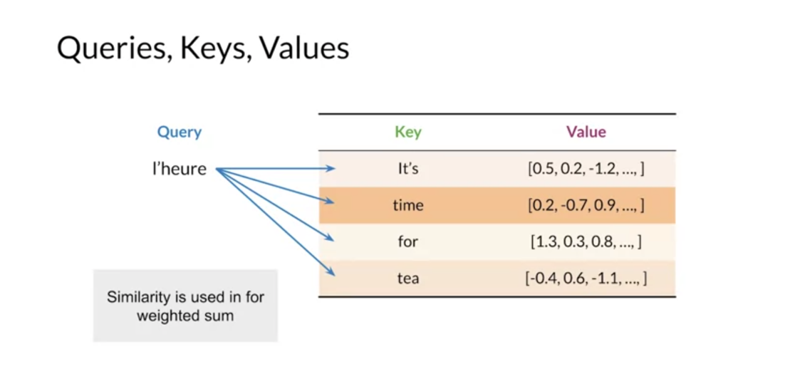
works as well as the concept of alignments between languages. Conceptually, you can think of keys and
values as a look up table. The query is matched to a key and the value associated with
that key is returned. For example,
if we are translating between french and english heure matches with time. So we’d like to get the value for
time, in practice to the queries, keys and
values are all represented by vectors. Embedding vectors for example.
Due to this, you don’t get exact matches
but the model can learn which words are the most similar between
the source and target languages. The similarity between
words is called alignment. The query and key vectors are used
to calculate alignment scores that are measures of how well the query and
keys match. These alignment scores are then
turned into weights used for a weighted sum of the value vectors, this weighted sum of the value vectors
is returned as the attention vector.
This process can be performed
using scale dot-product attention. The queries for each step are packed
together into a matrix Q. So attention can be computed
simultaneously for each query. The keys and values are also
packed into matrices K and V. These matrices are the inputs for the
attention function shown as a diagram on the left and mathematically on the rights. First, the queries and keys matrices are multiplied together
to get a matrix of alignments course. These are then scaled by the square
root of the key vector dimension, dk the scaling improves
the model performance for larger model sizes and could be
seen as a regularization constants. Next the scale scores are converted to
weights using the softmax function. Such that the weights for
each query sum to one. Finally the weights and the value matrices
are multiplied to get the attention vectors for each query, you can think of
the keys and the values as being the same. So when you multiply the softmax
output with V you are taking a linear combination of your initial input which
is then being fed to the decoder. Take a minute to make sure
what I just said makes sense.
No, that unlike the original form of
attention, scale dot-product attention consists of only two Matrix
multiplications and no neural networks. Since matrix multiplication is highly
optimized in modern deep learning frameworks. This form of attention is
much faster to compute but this also means that the alignments
between the source and target languages must
be learned elsewhere. Typically, alignment is learned
in the input embeddings or in other linear layers
before the attention layer.

Before moving on,
I want to look a bit closer at alignment. The alignment weights form a matrix with
queries, targets words on the rows and keys or source words on the columns. Each entry in this matrix is
the weight for the correspondent query, key pair word pairs that have similar
meanings, K and T, for example, will have larger weights than
the similar words like day and time. Through training, the model learns
which words have similar meanings and encodes that information and
the query and key vectors.

Learning alignment like
this is beneficial for translating between languages with
different grammatical structures. Since attention looks at the entire
input and target sentences at once and calculates alignments based on word pairs, weights are assigned appropriately
regardless of word order. For example, In the sentence, the
agreement on the European Economic Area was signed in August 1992 and this other
sentence lack of lasagne economic open. I mean you’re not meeting of sangatte
revenues, you can see that zone in the area are at different positions,
let’s have the same meaning. The model has learned to align them
appropriately, allowing the decoder to focus on the appropriate inputs
words despite different ordering.

Congrats on absorbing
all these new concepts. I introduced you to the purpose
of an attention layer. You saw how it is related with
information retrieval and I showed you how well it works even for
languages with very different structures. In the next video, I’ll be talking
about neural machine translation and show you what the setup looks like for
the system. I’ll show you what the data set looks
like and the steps required for pre processing your data sets. You have now seen what key square ease and
values are. These are important because if
you read a research paper you might come across these terms and
you will understand them. In the next video. I will talk about the setup for
machine translation.


Ungraded Lab: Scaled Dot-Product Attention
Scaled Dot-Product Attention: Ungraded Lab
The 2017 paper Attention Is All You Need introduced the Transformer model and scaled dot-product attention, sometimes also called QKV (Queries, Keys, Values) attention. Since then, Transformers have come to dominate large-scale natural language applications. Scaled dot-product attention can be used to improve seq2seq models as well. In this ungraded lab, you’ll implement a simplified version of scaled dot-product attention and replicate word alignment between English and French, as shown in Bhadanau, et al. (2014).
The Transformer model learns how to align words in different languages. You won’t be training any weights here, so instead you will use pre-trained aligned word embeddings from here. Run the cell below to load the embeddings and set up the rest of the notebook.
This is a practice notebook, where you can train writing your code. All of the solutions are provided at the end of the notebook.
# Import the libraries
import pickle
import matplotlib.pyplot as plt
import numpy as np

# Load the word2int dictionaries
with open("./data/word2int_en.pkl", "rb") as f:
    en_words = pickle.load(f)

with open("./data/word2int_fr.pkl", "rb") as f:
    fr_words = pickle.load(f)

# Load the word embeddings
en_embeddings = np.load("./data/embeddings_en.npz")["embeddings"]
fr_embeddings = np.load("./data/embeddings_fr.npz")["embeddings"]
# Define some helper functions

def tokenize(sentence, token_mapping):
    tokenized = []

    for word in sentence.lower().split(" "):
        try:
            tokenized.append(token_mapping[word])
        except KeyError:
            # Using -1 to indicate an unknown word
            tokenized.append(-1)

    return tokenized


def embed(tokens, embeddings):
    embed_size = embeddings.shape[1]

    output = np.zeros((len(tokens), embed_size))
    for i, token in enumerate(tokens):
        if token == -1:
            output[i] = np.zeros((1, embed_size))
        else:
            output[i] = embeddings[token]

    return output
The scaled-dot product attention consists of two matrix multiplications and a softmax scaling as shown in the diagram below from Vaswani, et al. (2017). It takes three input matrices, the queries, keys, and values.
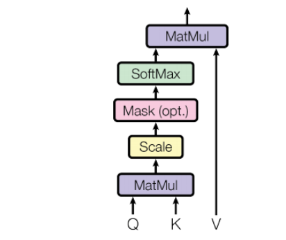
Mathematically, this is expressed as
A t t e n t i o n ( Q , K , V ) = s o f t m a x ( Q K ⊤ d k ) V \large \mathrm{Attention}\left(Q, K, V\right) = \mathrm{softmax}\left(\frac{QK^{\top}}{\sqrt{d_k}}\right)V Attention(Q,K,V)=softmax(dkQK⊤)V
where Q Q Q, K K K, and V V V are the queries, keys, and values matrices respectively, and d k d_k dk is the dimension of the keys. In practice, Q, K, and V all have the same dimensions. This form of attention is faster and more space-efficient than what you implemented before since it consists of only matrix multiplications instead of a learned feed-forward layer.
Conceptually, the first matrix multiplication is a measure of the similarity between the queries and the keys. This is transformed into weights using the softmax function. These weights are then applied to the values with the second matrix multiplication resulting in output attention vectors. Typically, decoder states are used as the queries while encoder states are the keys and values.
Exercise 1
Implement the softmax function with Numpy and use it to calculate the weights from the queries and keys. Assume the queries and keys are 2D arrays (matrices). Note that since the dot-product of Q and K will be a matrix, you’ll need to calculate softmax over a specific axis. See the end of the notebook for solutions.
def softmax(x, axis=0):
    """ Calculate softmax function for an array x

        axis=0 calculates softmax across rows which means each column sums to 1
        axis=1 calculates softmax across columns which means each row sums to 1
    """
    # Replace pass with your code.
    y = np.exp(x)
    return y / np.expand_dims(np.sum(y, axis=axis), axis)

def calculate_weights(queries, keys):
    """ Calculate the weights for scaled dot-product attention"""
    # Replace None with your code.
    dot = np.dot(queries, keys.T)/ np.sqrt(keys.shape[1])
    weights = softmax(dot, axis=1)

    assert weights.sum(axis=1)[0] == 1, "Each row in weights must sum to 1"

    # Replace pass with your code.
    return weights
在这段代码中,np.sum(y, axis=axis)计算了y数组沿着指定轴的和。然后,np.expand_dims()函数用于在这个和的基础上扩展一个维度,使得结果与y数组具有相同的维度,但在指定的轴上增加了一个长度为1的维度。
具体来说,假设y是一个二维数组,axis=1。np.sum(y, axis=1)将对每一行求和,得到一个形状为(y.shape[0],)的一维数组。然后,np.expand_dims(np.sum(y, axis=1), axis=1)将这个一维数组在第二个轴上扩展,得到一个形状为(y.shape[0], 1)的二维数组,其中每行的和仍然保持不变。
这个操作通常用于在计算softmax函数时,将每个元素除以对应行(或列)的总和,以确保每行(或列)的元素之和为1。这是因为softmax函数的结果通常被解释为概率分布,所以每行(或列)的和应该为1。
# Tokenize example sentences in English and French, then get their embeddings
sentence_en = "The agreement on the European Economic Area was signed in August 1992 ."
tokenized_en = tokenize(sentence_en, en_words)
embedded_en = embed(tokenized_en, en_embeddings)

sentence_fr = "L accord sur la zone économique européenne a été signé en août 1992 ."
tokenized_fr = tokenize(sentence_fr, fr_words)
embedded_fr = embed(tokenized_fr, fr_embeddings)

# These weights indicate alignment between words in English and French
alignment = calculate_weights(embedded_fr, embedded_en)

# Visualize weights to check for alignment
fig, ax = plt.subplots(figsize=(7,7))
ax.imshow(alignment, cmap='gray')
ax.xaxis.tick_top()
ax.set_xticks(np.arange(alignment.shape[1]))
ax.set_xticklabels(sentence_en.split(" "), rotation=90, size=16);
ax.set_yticks(np.arange(alignment.shape[0]));
ax.set_yticklabels(sentence_fr.split(" "), size=16);
If you implemented the weights calculations correctly, the alignment matrix should look like this:
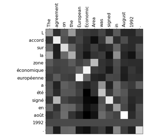
This is a demonstration of alignment where the model has learned which words in English correspond to words in French. For example, the words signed and signé have a large weight because they have the same meaning. Typically, these alignments are learned using linear layers in the model, but you’ve used pre-trained embeddings here.
Exercise 2
Complete the implementation of scaled dot-product attention using your calculate_weights function (ignore the mask).
def attention_qkv(queries, keys, values):
    """ Calculate scaled dot-product attention from queries, keys, and values matrices """

    # Replace pass with your code.
    attention = np.dot(calculate_weights(queries, keys), values)
    return attention


attention_qkv_result = attention_qkv(embedded_fr, embedded_en, embedded_en)

print(f"The shape of the attention_qkv function is {attention_qkv_result.shape}")
print(f"Some elements of the attention_qkv function are \n{attention_qkv_result[0:2,:10]}")
Output
The shape of the attention_qkv function is (14, 300)
Some elements of the attention_qkv function are
[[-0.04039161 -0.00275749  0.00389873  0.04842744 -0.02472726  0.01435613
  -0.00370253 -0.0619686  -0.00206159  0.01615228]
 [-0.04083253 -0.00245985  0.00409068  0.04830341 -0.02479128  0.01447497
  -0.00355203 -0.06196036 -0.00241327  0.01582606]]
Expected output
The shape of the attention_qkv function is (14, 300)
Some elements of the attention_qkv function are
[[-0.04039161 -0.00275749  0.00389873  0.04842744 -0.02472726  0.01435613
  -0.00370253 -0.0619686  -0.00206159  0.01615228]
 [-0.04083253 -0.00245985  0.00409068  0.04830341 -0.02479128  0.01447497
  -0.00355203 -0.06196036 -0.00241327  0.01582606]]
Solutions
def softmax(x, axis=0):
    """ Calculate softmax function for an array x

        axis=0 calculates softmax across rows which means each column sums to 1
        axis=1 calculates softmax across columns which means each row sums to 1
    """
    y = np.exp(x)
    return y / np.expand_dims(np.sum(y, axis=axis), axis)

def calculate_weights(queries, keys):
    """ Calculate the weights for scaled dot-product attention"""
    dot = np.matmul(queries, keys.T)/np.sqrt(keys.shape[1])
    weights = softmax(dot, axis=1)

    assert weights.sum(axis=1)[0] == 1, "Each row in weights must sum to 1"

    return weights

def attention_qkv(queries, keys, values):
    """ Calculate scaled dot-product attention from queries, keys, and values matrices """
    weights = calculate_weights(queries, keys)
    return np.matmul(weights, values)
Setup for Machine Translation
You will now learn about
how words are being represented in the neural
machine translation setting. You will also see what
the dataset looks like. When implementing
the systems I’ll show you that you need to
keep track of a few things. For example, which words
correspond to what sectors. With that said let’s dive in. This is an example
of the type of input data that you will have for your
assignments this week. Over here you have the
sequence, I’m hungry, and on the right you have the corresponding
French equivalent. Further down, I watch the soccer game and the
corresponding French equivalent. You’re going to have a
great many of these inputs. You should know
that the state of the art models use
pretrained vectors. But otherwise, the first
thing you’ll do is to use a one-hot vector
to represent the words. Usually you’ll keep track of your mappings with
the word to index, and index to word dictionary. Given any input, you
transform it into indices and then vice versa when you make
the predictions. You’ll also normally use
an end of sequence token. You will pad your token vectors with zeros to match the length of the longest sequence.

Here’s an example. This is an English sentence and the tokenized version of
the English sentence. You can see that
it has an index of 4,546 for the word both. After the initial tokenization, just add EOS token
shown here is one, and pad with zeros to match the length of
the longest sequence. Now let’s go to the
French translation of that sequence along with the tokenized version of
the French translation. Notice that one is the end
of sentence token here to. It’s also followed by a
series of padding zeros. Given now that you know
how to represent words, how to initialize your model, and how to structure
your dataset, you can go ahead and start
training your model. In the next video, I’ll show
you how you can do this.
Teacher Forcing
Hello. You’ll now learn how to train your neural machine
translation system. You will learn about
certain concepts like teacher forcing, and you’ll see some of its
advantages. Let’s dive in. In this section, you’ll see how to train your neural
machine translation, NMT for sorts, model
with attention. I’ll introduce you to the
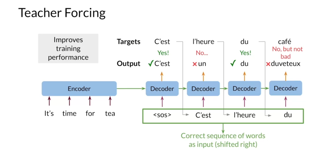
concepts of teacher forcing. As you learned before, seek to seek models generate
translations by feeding the output of the decoder
back in as the next inputs. This way there is no set
length on the output sequence. When training the
model, intuitively, you would compare the
decoder output sequence with the target sequence
to calculate the loss. That is, you would calculate the cross entropy
loss for each step, then sum the steps together
for the total loss. However, in practice, this
doesn’t work too well. The problem is that in the
early stages of training, the model is naive. It’ll make wrong predictions
early in the sequence. This problem compounds as the model keeps making
wrong predictions and the translated sequence gets further and further from
the target sequence.

The problem is illustrated
in this slide, where the final
outputs word duveteux has a similar word to the
word fluffy in English, which has a very different
meaning from the word team. To avoid this problem, you can use the
ground truth words as decoder inputs instead
of the decoder outputs. Even if the model makes
a wrong prediction, it pretends as if it’s made the correct one and
this can continue. This method makes training much faster and has a special
name, teacher forcing. There are some
variations on this tool. For example, you can slowly start using decoder
outputs over time, so that leads into training, you are no longer feeding
in the target words. This is known as
curriculum learning. You are now familiar
with teacher forcing, and you can add this
technique to your toolbox, to help you with
training your model, and to help you get
a better accuracy.
Teacher forcing 是一种训练循环神经网络(RNN)等序列模型的技术,它在训练过程中使用真实的(或者模型自己生成的)前一步输出作为当前步的输入,而不是使用上一步的预测结果。这样可以加快模型的训练速度和提高收敛性,尤其是在训练初期。
在使用Teacher forcing时,模型在训练过程中可以更快地学习到输入序列和输出序列之间的映射关系,因为它可以直接观察到正确的输出。然而,这种方法也存在一个问题,就是在实际推理阶段(即不使用Teacher forcing时),因为模型在训练过程中始终依赖于前一步的真实输出,可能导致模型在推理阶段表现不佳,即所谓的“曝光偏差”(exposure bias)问题。
为了解决这个问题,可以在训练过程中以一定的概率使用模型自己生成的前一步输出作为当前步的输入,这样可以更好地模拟实际推理时的情况,称为“Scheduled Sampling”。通过逐渐增加使用模型自己生成的输出的概率,可以平衡训练和推理之间的差异,提高模型在推理阶段的性能。
NMT Model with Attention
Welcome. I will now
show you how to train a neural machine
translation system from scratch. I’ll go through every step
slowly so you can understand what is going on behind the
scenes. Let’s get started. In this video, I’ll show you how everything you have
seen this week fits together into the
model architecture you will implement in
this week’s assignments. First, I’ll give you
a general overview before I go into the
more intricate details. You will implement
a model similar to the one you have seen
in previous lectures. You will have an encoder that
gets the input sequence, a decoder which is supposed
to do the translation, and an Attention Mechanism
which would help the decoder focus on the important parts of
the input sequence. Recall that the decoder
is supposed to pass hidden states to the
Attention Mechanism to get context vectors. The pass of the hidden
states from the decoder to the Attention Mechanism could
not be easy to implement. Instead, you will be
using two decoders, a pre-attention decoder
to provide hidden states, and a post-attention decoder which will provide
the translation.

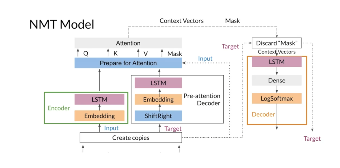
A general overview of the modified model
looks as follows. You will have the encoder
and a pre-attention decoder that’s got the inputs
and target sequences. Then for the
pre-attention decoder, the target sequence
is shifted right, which is how you’ll be
implementing the teacher forcing. From the encoder and
pre-attention decoder, you will retrieve
the hidden states at each step and use them as inputs for the
Attention Mechanism. You will use the
hidden states from the encoder as the
keys and values, while those from the
decoder are the queries. As you have seen in
previous lectures, the Attention Mechanism will use these values to compute
the context vectors. Finally, the post-attention
decoder will use the context vectors as inputs to provide the
predicted sequence.

Now, let’s take a closer look at each piece of the model. The initial step is
to make two copies of the input tokens and
the target tokens because you will need them in different places of the model. One copy of the input tokens
is fed into the encoder, which is used to transform them into the key
and value vectors, while a copy of
the target tokens goes into the
pre-attention decoder. Note that the
computations done in the encoder and
pre-attention decoder could be done in parallel, since they don’t
depend on each other. Within the
pre-attention decoder, you shift each
sequence to the right and add a start of
sentence token. In the encoder and
pre-attention decoder, the inputs and
targets go through an embedding layer
before going to LSTMs. After getting the query
key and value vectors, you have to prepare them
for the attention layer. You’ll use a function
to help you get a padding mask to help the attention layer determine
the padding tokens. This step is where you will use the copy of
the input tokens. Now, everything is
ready for attention. You pass the queries,
keys, values, and the mask to the
attention layer that outputs the context
vector and the mask. Before going through the
decoder, you drop the mask. You then pass the
context vectors through the decoder composed of an LSTM, a dense layer, and a LogSoftmax. In the end, your model returns log probabilities and the copy of the target tokens that
you made at the beginning. There you have it,
the model you’ll be building and the intuition
behind all the steps. Take a break and just
let all that sink in. You now have an overview
of how NMT is implemented. If you did not
understand everything, do not worry about it. We will go in more detail in this week’s programming
assignments. In the next video, I will talk about how to
evaluate your system.
BLEU Score
After building and
training your model, it is essential to assess
how well it performs. For machine translation, you have different metrics that were engineered
just for this task. In this lecture, I will
show you the BLEU score and some of its issues
for evaluating machine translation models. The BLEU score, a bilingual
evaluation under study, is an algorithm designed
to evaluate some of the most challenging problems in NLP, including
machine translation. It evaluates the quality of
machine-translated text by comparing a candidate
translation to one or more references, which are often
human translations. The closer the BLEU
score is to one, the better your model is, the closer to zero,
the worse it is.

With that said, what is the BLEU score and why is
this an important metric? To get the BLEU score, you have to compute the
precision of the candidates by comparing its end-grams
with reference translations. To demonstrate, I’ll use
unigrams as an example. Let’s say that you have a
candidate sequence that you got from your model
composed of I, I, am, I. You also have one
reference translation which contains the words, Eunice said, I’m hungry. A second reference translation
that includes the words, he said, I’m hungry. To get the BLEU score, you count how many words from the candidate appear in any of the references and
divide that count by the total number of words in
the candidate translation. You can view it as
a precision metric.

You have to go
through all the words in the candidate translation. First, you have the word I, which appears in both
reference translations. You add one to your count. Then you have again the word I, which you already know
appears on both references, and you add one to your count. After that, you have the word am which also appears
in both references. You add that word to your count. At the end, you have
the word I again, which appears on
both references. You can add one to your count. Finally, you can get the
BLEU score by dividing your count by the number of words in the candidate
translation, which in this case
is equal to 4. The whole process gives you
a BLEU score equal to 1. Weird? This translation that is far from being equal to the references got
a perfect score. With this vanilla BLEU score, a model that always outputs
common words will do great.

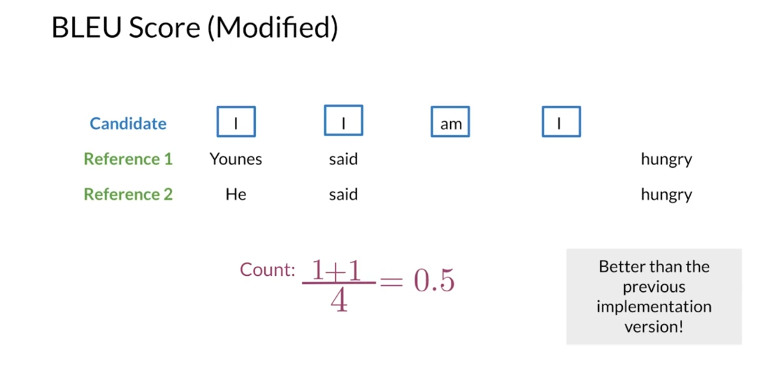
Let’s try a modified
version that will give you a better estimate of
your model’s performance. For the modified version
of the BLEU score, after you find a word from the candidates in one or
more of the references, you stop considering
that word from the reference for the following
words in the candidates. In other words, you
exhaust the words in the references after you match them with a word
in the candidates. Let’s start from the beginning of the candidate translation. You have the word I that
appears in both references. You add one to your count and exhaust the word I
from both references. Then you have the word I again, but you don’t have that word
in the references because it was taken out for the
previous word in the candidate. You don’t add anything
to your count. Then you have the word M, which appears in
both references. You add one to your counts and eliminate the word M
from both references. After that, you have
the word I again, but no left occurrences
in the references. You don’t add anything
to your counts. Finally, you divide your count
by the number of words in the candidate translation
to get BLEU score of 2/4 or 0.5. As you can note, this version of the BLEU score makes more sense than the vanilla implementation.
However, like anything in life, using the BLEU score as an evaluation metric
has some caveats. For one, it doesn’t consider the semantic
meaning of the words. It also doesn’t consider the
structure of the sentence. Imagine getting
this translation. Ate I was hungry because. If the reference sentence is
I ate because I was hungry, this would get a
perfect BLEU score. BLEU score is the most widely
adopted evaluation metric for machine translation. But you should be aware of these drawbacks before using it.

You now know how to evaluate your machine translation
model using the BLEU score. I also showed you that this
metric has some issues because it doesn’t care about semantics and
sentence structure. In the following video, you’ll see another metric
for machine translation. That metric could be used to better estimate your
model performance.
BLEU(Bilingual Evaluation Understudy)和ROUGE(Recall-Oriented Understudy for Gisting Evaluation)都是用于评估自然语言处理任务中生成文本质量的指标,但它们在应用和计算方式上有一些不同之处。
用途:
- BLEU主要用于机器翻译任务,用于评估机器翻译系统生成的译文与参考译文之间的相似程度。
- ROUGE主要用于文本摘要任务,用于评估生成的摘要与参考摘要之间的相似程度。
计算方式:
- BLEU通过比较候选译文中的n-gram与参考译文中的n-gram的匹配情况来计算得分。它计算了n-gram的精确匹配率,并使用一个惩罚项来惩罚过度短的译文。
- ROUGE使用类似的方法,但通常使用的是召回率(Recall)作为评估指标,因为在文本摘要任务中,关键信息的召回更为重要。
评价指标:
- BLEU的评价指标是介于0到1之间的值,接近1表示候选译文与参考译文之间的相似度更高。
- ROUGE通常包括多个指标,如ROUGE-N(N-gram级别的召回率)、ROUGE-L(最长公共子序列级别的召回率)等,也是介于0到1之间的值,值越高表示生成的摘要与参考摘要之间的相似度更高。
总的来说,BLEU和ROUGE都是用于评估生成文本质量的重要指标,但它们适用于不同的任务,并且在计算方式和评价指标上存在一些差异。
Ungraded Lab: BLEU Score
Calculating the Bilingual Evaluation Understudy (BLEU) score: Ungraded Lab
In this ungraded lab, you will implement a popular metric for evaluating the quality of machine-translated text: the BLEU score proposed by Kishore Papineni, et al. in their 2002 paper “BLEU: a Method for Automatic Evaluation of Machine Translation”. The BLEU score works by comparing a “candidate” text to one or more “reference” texts. The score is higher the better the result. In the following sections you will calculate this value using your own implementation as well as using functions from a library.
1. Importing the Libraries
You will start by importing the Python libraries. First, you will implement your own version of the BLEU Score using NumPy. To verify that your implementation is correct, you will compare the results with those generated by the SacreBLEU library. This package provides hassle-free computation of shareable, comparable, and reproducible BLEU scores. It also knows all the standard test sets and handles downloading, processing, and tokenization.
import numpy as np                  # import numpy to make numerical computations.
import nltk                         # import NLTK to handle simple NL tasks like tokenization.
nltk.download("punkt")
from nltk.util import ngrams
from collections import Counter     # import a counter.
!pip3 install 'sacrebleu'           # install the sacrebleu package.
import sacrebleu                    # import sacrebleu in order compute the BLEU score.
import matplotlib.pyplot as plt     # import pyplot in order to make some illustrations.
2. BLEU score
2.1 Definitions and formulas
You have seen how to calculate the BLEU score in this week’s lectures. Formally, you can express the BLEU score as:
B L E U = B P × ( ∏ i = 1 n p r e c i s i o n i ) ( 1 / n ) . (1) BLEU = BP\times\Bigl(\prod_{i=1}^{n}precision_i\Bigr)^{(1/n)}.\tag{1} BLEU=BP×(i=1∏nprecisioni)(1/n).(1)
The BLEU score depends on the B P BP BP, which stands for Brevity Penalty, and the weighted geometric mean precision for different lengths of n-grams, both of which are described below. The product runs from i = 1 i=1 i=1 to i = n i=n i=n to account for 1-grams to n-grams and the exponent of 1 / n 1/n 1/n is there to calculate the geometrical average. In this notebook, you will use n = 4 n=4 n=4
The Brevity Penalty is defined as an exponential decay:
B P = m i n ( 1 , e ( 1 − ( l e n ( r e f ) / l e n ( c a n d ) ) ) ) , (2) BP = min\Bigl(1, e^{(1-({len(ref)}/{len(cand)}))}\Bigr),\tag{2} BP=min(1,e(1−(len(ref)/len(cand)))),(2)
where l e n ( r e f ) {len(ref)} len(ref) and l e n ( c a n d ) {len(cand)} len(cand) refer to the length or count of words in the reference and candidate translations. The brevity penalty helps to handle very short translations.
The precision is defined as :
p r e c i s i o n i = ∑ s i ∈ c a n d m i n ( C ( s i , c a n d ) , C ( s i , r e f ) ) ∑ s i ∈ c a n d C ( s i , c a n d ) . (3) precision_i = \frac {\sum_{s_i \in{cand}}min\Bigl(C(s_i, cand), C(s_i, ref)\Bigr)}{\sum_{s_i \in{cand}} C(s_i, cand)}.\tag{3} precisioni=∑si∈candC(si,cand)∑si∈candmin(C(si,cand),C(si,ref)).(3)
The sum goes over all the i-grams s i s_i si in the candidate sentence c a n d cand cand. C ( s i , c a n d ) C(s_i, cand) C(si,cand) and C ( s i , r e f ) C(s_i, ref) C(si,ref) are the counts of the i-grams in the candidate and reference sentences respectively. So the sum counts all the n-grams in the candidate sentence that also appear in the reference sentence, but only counts them as many times as they appear in the reference sentence and not more. This is then divided by the total number of i-grams in the candidate sentence.
2.2 Visualizing the BLEU score
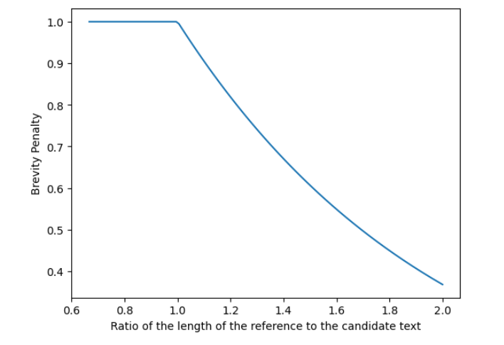
Brevity Penalty:
The brevity penalty penalizes generated translations that are shorter than the reference sentence. It compensates for the fact that the BLEU score has no recall term.
reference_length = 1
candidate_length = np.linspace(1.5, 0.5, 100)

length_ratio = reference_length / candidate_length
BP = np.minimum(1, np.exp(1 - length_ratio))

# Plot the data
fig, ax = plt.subplots(1)
lines = ax.plot(length_ratio, BP)
ax.set(
    xlabel="Ratio of the length of the reference to the candidate text",
    ylabel="Brevity Penalty",
)
plt.show()
Output
N-Gram Precision:
The n-gram precision counts how many n-grams (in your case unigrams, bigrams, trigrams, and four-grams for i =1 , … , 4) match their n-gram counterpart in the reference translations. This term acts as a precision metric. Unigrams account for adequacy while longer n-grams account for fluency of the translation. To avoid overcounting, the n-gram counts are clipped to the maximal n-gram count occurring in the reference ( m n r e f m_{n}^{ref} mnref). Typically precision shows exponential decay with the degree of the n-gram.
# Mocked dataset showing the precision for different n-grams
data = {"1-gram": 0.8, "2-gram": 0.7, "3-gram": 0.6, "4-gram": 0.5}

# Plot the datapoints defined above
fig, ax = plt.subplots(1)
bars = ax.bar(*zip(*data.items()))
ax.set(ylabel="N-gram precision")
plt.show()
Output

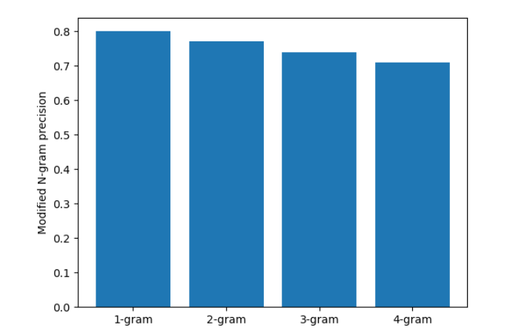
N-gram BLEU score:
When the n-gram precision is normalized by the brevity penalty (BP), then the exponential decay of n-grams is almost fully compensated. The BLEU score corresponds to a geometric average of this modified n-gram precision.
# Mocked dataset showing the precision multiplied by the BP for different n-grams
data = {"1-gram": 0.8, "2-gram": 0.77, "3-gram": 0.74, "4-gram": 0.71}

# Plot the datapoints defined above
fig, ax = plt.subplots(1)
bars = ax.bar(*zip(*data.items()))
ax.set(ylabel="Modified N-gram precision")
plt.show()
Output
3. Example Calculations of the BLEU score
In this example you will have a reference sentence and 2 candidate sentences. You will tokenize all sentences using the NLTK package. Then you will compare the two candidates to the reference using BLEU score.
First you define and tokenize the sentences.
reference = "The NASA Opportunity rover is battling a massive dust storm on planet Mars."
candidate_1 = "The Opportunity rover is combating a big sandstorm on planet Mars."
candidate_2 = "A NASA rover is fighting a massive storm on planet Mars."

tokenized_ref = nltk.word_tokenize(reference.lower())
tokenized_cand_1 = nltk.word_tokenize(candidate_1.lower())
tokenized_cand_2 = nltk.word_tokenize(candidate_2.lower())

print(f"{reference} -> {tokenized_ref}")
print("\n")
print(f"{candidate_1} -> {tokenized_cand_1}")
print("\n")
print(f"{candidate_2} -> {tokenized_cand_2}")
Output
The NASA Opportunity rover is battling a massive dust storm on planet Mars. -> ['the', 'nasa', 'opportunity', 'rover', 'is', 'battling', 'a', 'massive', 'dust', 'storm', 'on', 'planet', 'mars', '.']


The Opportunity rover is combating a big sandstorm on planet Mars. -> ['the', 'opportunity', 'rover', 'is', 'combating', 'a', 'big', 'sandstorm', 'on', 'planet', 'mars', '.']


A NASA rover is fighting a massive storm on planet Mars. -> ['a', 'nasa', 'rover', 'is', 'fighting', 'a', 'massive', 'storm', 'on', 'planet', 'mars', '.']
3.1 Define the functions to calculate the BLEU score
Computing the Brevity Penalty
You will start by defining the function for brevity penalty according to the equation (2) in section 2.1.
def brevity_penalty(candidate, reference):
    """
    Calculates the brevity penalty given the candidate and reference sentences.
    """
    reference_length = len(reference)
    candidate_length = len(candidate)

    if reference_length < candidate_length:
        BP = 1
    else:
        penalty = 1 - (reference_length / candidate_length)
        BP = np.exp(penalty)

    return BP
Computing the clipped Precision
Next, you need to define a function to calculate the geometrically averaged clipped precision. This function calculates how many of the n-grams in the candidate sentence actually appear in the reference sentence. The clipping takes care of overcounting. For example if a certain n-gram appears five times in the candidate sentence, but only twice in the reference, the value is clipped to two.
def average_clipped_precision(candidate, reference):
    """
    Calculates the precision given the candidate and reference sentences.
    """

    clipped_precision_score = []

    # Loop through values 1, 2, 3, 4. This is the length of n-grams
    for n_gram_length in range(1, 5):
        reference_n_gram_counts = Counter(ngrams(reference, n_gram_length))
        candidate_n_gram_counts = Counter(ngrams(candidate, n_gram_length))

        total_candidate_ngrams = sum(candidate_n_gram_counts.values())

        for ngram in candidate_n_gram_counts:
            # check if it is in the reference n-gram
            if ngram in reference_n_gram_counts:
                # if the count of the candidate n-gram is bigger than the corresponding
                # count in the reference n-gram, then set the count of the candidate n-gram
                # to be equal to the reference n-gram

                if candidate_n_gram_counts[ngram] > reference_n_gram_counts[ngram]:
                    candidate_n_gram_counts[ngram] = reference_n_gram_counts[ngram] # t

            else:
                candidate_n_gram_counts[ngram] = 0 # else set the candidate n-gram equal to zero

        clipped_candidate_ngrams = sum(candidate_n_gram_counts.values())

        clipped_precision_score.append(clipped_candidate_ngrams / total_candidate_ngrams)

    # Calculate the geometric average: take the mean of elemntwise log, then exponentiate
    # This is equivalent to taking the n-th root of the product as shown in equation (1) above
    s = np.exp(np.mean(np.log(clipped_precision_score)))

    return s
reference_n_gram_counts = Counter(ngrams(reference, n_gram_length)) 解释
这段代码使用了 NLTK(Natural Language Toolkit)和 Python 的 collections 模块来计算参考文本(reference)中 n 元组(n-grams)的数量。下面对每一行进行解释:
from nltk.util import ngrams: 这行代码从 NLTK 工具包中导入了 ngrams 函数,该函数用于生成文本的 n 元组序列。from collections import Counter: 这行代码从 Python 的 collections 模块中导入了 Counter 类,用于计算可哈希对象的频率。reference_n_gram_counts = Counter(ngrams(reference, n_gram_length)): 这行代码计算了参考文本中 n 元组的数量,并将结果存储在 reference_n_gram_counts 变量中。具体地,它使用了 ngrams 函数生成了 reference 中的所有 n 元组,并使用 Counter 类对这些 n 元组进行计数。这样,reference_n_gram_counts 就是一个包含了参考文本中所有 n 元组及其出现次数的字典。
Computing the BLEU score
Finally, you can compute the BLEU score using the above two functions.
def bleu_score(candidate, reference):
    BP = brevity_penalty(candidate, reference)
    geometric_average_precision = average_clipped_precision(candidate, reference)
    return BP * geometric_average_precision
3.2 Testing the functions
Now you can test the functions with your Example Reference and Candidates Sentences.
result_candidate_1 = round(bleu_score(tokenized_cand_1, tokenized_ref) * 100, 1)
print(f"BLEU score of reference versus candidate 1: {result_candidate_1}")
result_candidate_2 = round(bleu_score(tokenized_cand_2, tokenized_ref) * 100, 1)
print(f"BLEU score of reference versus candidate 2: {result_candidate_2}")
Output
BLEU score of reference versus candidate 1: 27.6
BLEU score of reference versus candidate 2: 35.3
3.3 Comparing the Results from your Code with the Sacrebleu Library
Below you will do the same calculation, but using the sacrebleu library. Compare them with your implementation above.
result_candidate_1 = round(sacrebleu.sentence_bleu(candidate_1, [reference]).score, 1)
print(f"BLEU score of reference versus candidate 1: {result_candidate_1}")
result_candidate_2 = round(sacrebleu.sentence_bleu(candidate_2, [reference]).score, 1)
print(f"BLEU score of reference versus candidate 2: {result_candidate_2}")
Output
BLEU score of reference versus candidate 1: 27.6
BLEU score of reference versus candidate 2: 35.3
4. BLEU computation on a corpus
4.1 Loading Datasets for Evaluation Using the BLEU Score
In this section, you will use a simple pipeline for evaluating machine translated text. You will use English to German translations generated by Google Translate. There are three files you will need:
- A source text in English. In this lab, you will use the first 1671 words of the wmt19 evaluation dataset downloaded via SacreBLEU.
- A reference translation to German of the corresponding first 1671 words from the original English text. This is also provided by SacreBLEU.
- A candidate machine translation to German from the same 1671 words. This is generated by Google Translate.
With that, you can now compare the reference and candidate translation to get the BLEU Score.
# Loading the raw data
wmt19_src = open("data/wmt19_src.txt", "r")
wmt19_src_1 = wmt19_src.read()
wmt19_src.close()

wmt19_ref = open("data/wmt19_ref.txt", "r")
wmt19_ref_1 = wmt19_ref.read()
wmt19_ref.close()

wmt19_can = open("data/wmt19_can.txt", "r")
wmt19_can_1 = wmt19_can.read()
wmt19_can.close()

tokenized_corpus_src = nltk.word_tokenize(wmt19_src_1.lower())
tokenized_corpus_ref = nltk.word_tokenize(wmt19_ref_1.lower())
tokenized_corpus_cand = nltk.word_tokenize(wmt19_can_1.lower())
Now that you have your data loaded, you can inspect the first sentence of each dataset.
print("English source text:\n")
print(f"{wmt19_src_1[0:170]} -> {tokenized_corpus_src[0:30]}\n\n")
print("German reference translation:\n")
print(f"{wmt19_ref_1[0:219]} -> {tokenized_corpus_ref[0:35]}\n\n")
print("German machine translation:\n")
print(f"{wmt19_can_1[0:199]} -> {tokenized_corpus_cand[0:29]}")
Output
English source text:

Welsh AMs worried about 'looking like muppets'
There is consternation among some AMs at a suggestion their title should change to MWPs (Member of the Welsh Parliament).
 -> ['\ufeffwelsh', 'ams', 'worried', 'about', "'looking", 'like', "muppets'", 'there', 'is', 'consternation', 'among', 'some', 'ams', 'at', 'a', 'suggestion', 'their', 'title', 'should', 'change', 'to', 'mwps', '(', 'member', 'of', 'the', 'welsh', 'parliament', ')', '.']


German reference translation:

Walisische Ageordnete sorgen sich "wie Dödel auszusehen"
Es herrscht Bestürzung unter einigen Mitgliedern der Versammlung über einen Vorschlag, der ihren Titel zu MWPs (Mitglied der walisischen Parlament) ändern soll.
 -> ['\ufeffwalisische', 'ageordnete', 'sorgen', 'sich', '``', 'wie', 'dödel', 'auszusehen', "''", 'es', 'herrscht', 'bestürzung', 'unter', 'einigen', 'mitgliedern', 'der', 'versammlung', 'über', 'einen', 'vorschlag', ',', 'der', 'ihren', 'titel', 'zu', 'mwps', '(', 'mitglied', 'der', 'walisischen', 'parlament', ')', 'ändern', 'soll', '.']


German machine translation:

Walisische AMs machten sich Sorgen, dass sie wie Muppets aussehen könnten
Einige AMs sind bestürzt über den Vorschlag, ihren Titel in MWPs (Mitglied des walisischen Parlaments) zu ändern.
Es ist aufg -> ['walisische', 'ams', 'machten', 'sich', 'sorgen', ',', 'dass', 'sie', 'wie', 'muppets', 'aussehen', 'könnten', 'einige', 'ams', 'sind', 'bestürzt', 'über', 'den', 'vorschlag', ',', 'ihren', 'titel', 'in', 'mwps', '(', 'mitglied', 'des', 'walisischen', 'parlaments']
And lastly, you can calculate the BLEU score of the translation.
result =  round(sacrebleu.sentence_bleu(wmt19_can_1, [wmt19_ref_1]).score, 1)
print(f"BLEU score of the reference versus candidate translation: {result}")
Output
BLEU score of the reference versus candidate translation: 43.2
4.2 BLEU Score Interpretation on a Corpus
The table below (taken from here) shows the typical values of BLEU score. You can see that the translation above is of high quality according to this table and in comparison to the given reference sentence. (if you see “Hard to get the gist”, please open your workspace, delete wmt19_can.txt and get the latest version via the Lab Help button)
| Score | Interpretation |
|---|---|
| < 10 | Almost useless |
| 10 - 19 | Hard to get the gist |
| 20 - 29 | The gist is clear, but has significant grammatical errors |
| 30 - 40 | Understandable to good translations |
| 40 - 50 | High quality translations |
| 50 - 60 | Very high quality, adequate, and fluent translations |
| > 60 | Quality often better than human |
ROUGE-N Score
Previously, I introduced you to the BLEU score evaluation metric and it’s
modified version. I used it to assess the performance of machine
translation models. I also showed you some
drawbacks that’s arise because that metric ignores semantic
and sentence structure. In this video, I’ll talk
about the ROUGE score, another performance
metric that tends to estimate the quality of
machine translation systems. I’ll introduce You now to a family of metrics
called ROUGE. It stands for
Recall-Oriented Understudy of Gisting Evaluation, which is a mouthful. But lets you know,
right off the bat, that it’s more
recall-oriented by default. That means that ROUGE cares
about how much of the human created references appear in
the candidate translation. In contrast, BLEU is
precision oriented. Since you have to
determine how many words from the candidates
appear on the references. ROUGE was initially
developed to evaluate the quality of the
machine summarized texts, but is also helpful in assessing the quality
of machine translation. It works by comparing the machine candidates against reference translations
provided by humans. There are many versions
of the ROUGE score, but also the one called
ROUGE-N. For the ROUGE-N score, You have to get the counts of the n-gram overlaps between the candidates and the
reference translations, which is somewhat
similar to what you have to do for
the BLEU score.
To see the difference
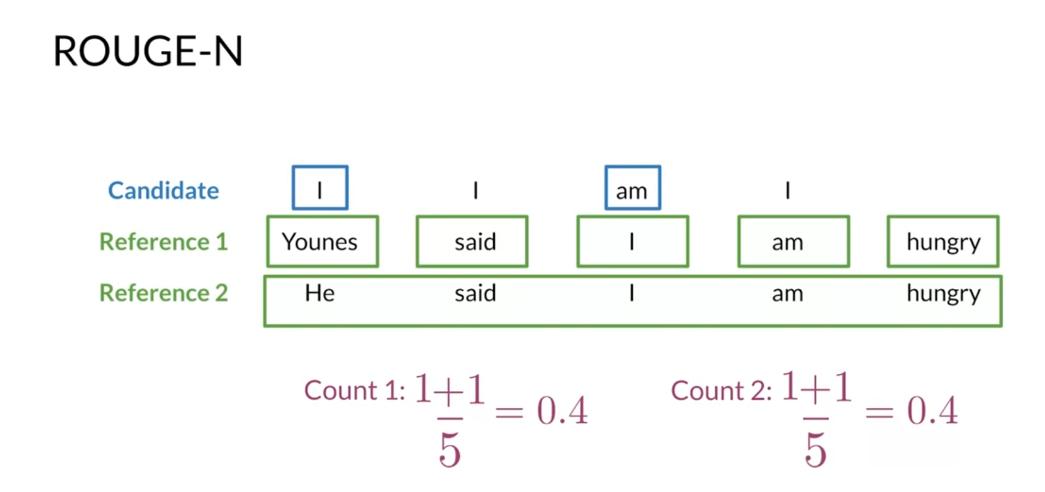
between the two metrics, I’ll show You an example of how ROUGE-N works with uni-grams. To get the basic version of the ROUGE-N score based only on recall so you must count word matches between the
reference and the candidates, and divide by the number
of words in the reference. If you had multiple references, you would need to get a ROUGE-N score using each
reference and get the maximum. Now, let’s go through
the example that you already solved
for the BLEU score. Your candidate has the
words I two times, the word M, and
the word I again, for a total of four words. You also have a
reference translation. Younes said, “I am hungry” and another slightly
different reference. He said, “I’m hungry.” Each reference has
five words in total. You have to count
matches between the references and the
candidate translations, similar to what you did
for the BLEU score. Let’s start with the
first reference. The word Younes, doesn’t match any of the uni-grams
in the candidates, so you don’t add
anything to the counts. The word said doesn’t match any word and the
candidates either. The word I, has
multiple matches, but you need the first one. For this match, you add
only one to your counts. The word M has a match in the candidates so your
increment your counts. Now, the final word of the
first reference, hungry, doesn’t match any of the
words from the candidates. You don’t add anything
to your counts. If you repeat this process
for the second reference, you get a counts equal to 2. Finally, you divide these
counts by the number of words in each reference
and get the maximum value, which for this example
is equal to 0.4.
This basic version of the
ROUGE-N score is based on recall while the BLEU score you saw in the previous
lectures is precision. But why not combine both to get a metric like an F1 score? Recall, pun intended, from your introductory
machine learning courses that the F1 score is given
by this formula, two times the product of
precision and recall, divided by the sum
of both metrics. You get the following formula, if you replace precision
by the modified version of the BLEU score and recall
by the ROUGE-N score. For this example, you have
a BLEU score equal to 0.5, which you got in
previous lectures. You have a ROUGE-N score
equivalent to 0.4, that you calculated before. With these values, you will have an F1 score equal to 4
over 9, close to 0.44. You have now seen how to compute the modified BLEU and the sample ROUGE-N scores
to evaluate your model. You can view these metrics
like precision and recall. Therefore, you can use both to get an F1
score that’s could better assess the performance of your machine
translation model. In many applications, you
will see reported and F-score along with the
BLEU and ROUGE-N metric. However, you must note that’s all the evaluation metrics
you have seen so far, don’t consider the sentence
structure and semantics, only accounts for
matching n-grams between candidates and the
reference translations.

You now have seen how to
compute the modified BLEU and the simple ROUGE-N scores
to evaluate your model. You can view these metrics
like precision and recall. Therefore, you can use both to get an F1 score that’s good, better assess the performance of your machine
translation model. In many applications,
you’ll see reported an F-score along with the
BLEU and the ROUGE-N metrics. However, you must note that all the evaluation
metrics you have seen so far don’t consider the sentence structure
and semantics. They only account
for matching n-grams between the candidates and
reference translations.
Sampling and Decoding
Hello. You will now learn about two ways that will allow you to construct a sentence. The first approach is known as greedy decoding and
the second approach is known as random sampling. You’ll also see the pros and
the cons of each method. For example, when
choosing the word with the highest probability
at every time step, that does not necessarily
generate the best sequence. With that said, let’s dive in and explore
these two methods. By now you have reached
the final parts of this week’s lectures.
That’s awesome. I’ll show you a few methods
for sampling and decoding, as well as a discussion of an important type of parameter in sampling called temperature. First, a quick reminder on how a seq2seq model
predicts words. The output of the
decoder is produced from a dense layer and a softmax
or log softmax operation. The output at each step then is the probability
distribution over all the words and symbols
in the target vocabulary. The final output of the
model depends on how you choose the words using these probability
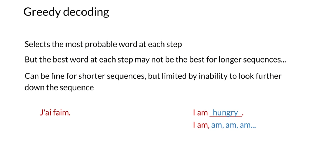
distributions at each step. Greedy decoding is the
simplest way to decode the model’s predictions
as it selects the most probable
word at every step. However, this approach
has limitations. When you consider the
highest probability for each prediction and concatenate all predicted tokens for the output sequence. As the greedy decoder does, you can end up with
a situation where the output instead of, “I am hungry,” gives you “I am, am, am” and so forth. You can see how this
could be a problem, but not in all cases. For shorter sequences,
it’s going to be fine. But if you have many
other words to consider, then knowing what’s
coming up next might help you better
predict the next sequence.
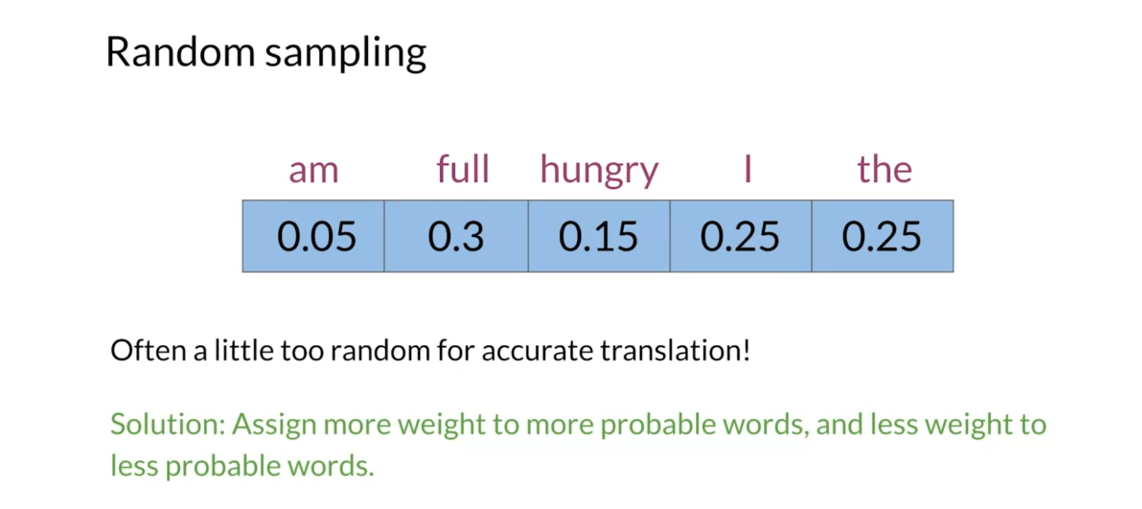
Another option is known
as random sampling. What random sampling
does is it provides probabilities for each word and sample accordingly
for the next outputs. One of the problems with this is that it could be a
little bit too random. A solution for this is to
assign more weight to the words with higher probabilities and
less weight to the others. You will see a method for doing this in just a few moment.
In sampling, temperature
is a parameter you can adjust to allow for more or less randomness
in your predictions. It’s measured on a scale of 0-1, indicating low to
high randomness. Let’s say you need your
model to make careful, safe decisions about
what to output. Then set you’re parameter lower and get the prediction
equivalent of a very confident but rather a boring person seated next to
you at a dinner table. If you feel like taking
more of a gamble, set your temperature
a bit higher. This has the effect of making
your network more excited. You may get some pretty
fun predictions. On the other hand, there will be probably a lot more mistakes.

You have seen in this video, methods for sampling
and decoding that will allow you to construct
sentences using your model. However, these methods don’t always produce the most
convincing outputs. Instead, you’ll often get a
very random set of words. In the next videos, you’ll see two methods
for sampling and decoding that tend to
produce better results.
Beam Search
Beam search is a technique that allows
you to find the best sequences over a fixed window size
known as the beam with. Since taking the output with the highest
probability at each time step is not ideal. I will show you how to
use beam search instead. So far the methods I’ve presented only
consider word probabilities one at a time. These ways of sampling might not result
in the highest probability sequences and the sentence is produced Using
these methods could not make sense. The overall most probable
translation given an input sentence is not necessarily the most
probable word at each step. For example, it’s possible that choosing
the most probable words at the start of the sequence could lead to
a worse translation compared to choosing in other words. If you had infinite computational power,
you could calculate the probabilities of every possible
output sentence and choose the best one. In the real world we use beam search. This method attempts to find the most
likely outsports sentence by choosing some number of best sequences based on
conditional probabilities at each time step.
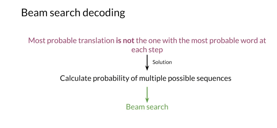
Now at each time step with beam search
you have to calculate the probability of potential sequences given the outputs
of the previous time step. To avoid computing the probability for every possible sequence you have
armature beam called the beam width. At each step, you only keep the most
probable sequences and drop all others. You generate a new word until all be most
probable sentences and with the US token. So beam search consumes
a lot of memory and could be computationally costly
depending on your choice for beam. As an interesting side note,
greedy decoding is just a particular case of beam search where you set
the beam with B to be equal to 1.
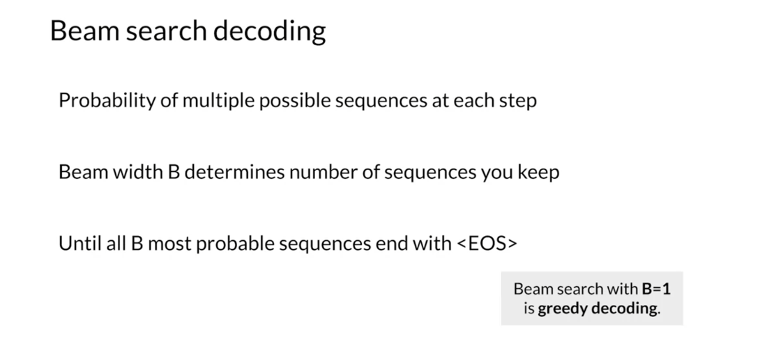
To illustrate this method,
consider a small vocabulary consisting of the words I am hungry and
an end of sentence token. And let’s say the beam
with B is equal to 2. As with the other methods beam search
starts with the start of sentence token and gets the probabilities for
the first word in the sequence. Here I has a probability of 0.5,
am has a probability of 0.4 and hungry has a probability of 0.1 and
in the eos is at 0. Since the beam with is 2 you keep
the two highest probabilities I and am. Then you calculate the conditional
probability of all other words Given the two sequences that
you have kept so far I and am. Given the word I, the model returns
am with a probability of 0.5 and hungry with 0.3. Given the words am,
the model returns the probability of word I with a probability of 0.7 and
hungry with a probability of 0.2. These are the two conditional
probabilities given the two previous sequences of B of word 2 given word 1. Next you calculate the probability
by multiplying the conditional probability for 2 given the word I
with the probability of words I. For instance if the sequence
of II has a probability of 0.5 times 0.1 this is equal to 0.05. The sequence I am has a probability of
0.5 times 0.5 which is equal to 0.25. You have to do the same with
the sequences starting with the word am. Here the sequence MI has a probability
of 0.4 times 0.7 which is equal to 0.28. At this point there is possible sequences
but with the beam width B=2 you only keep the two sequences with
the highest probabilities. So you keep the sequence I am and
am I and drop all others. Then for the next step you use am as
the inputs were to get the conditional probabilities for the I am sequence and
I for the am I sequence. You repeat the process to calculate
the joints probabilities and again choose the best sequence. This process stops with the model
predicts an end of sentence token for all, be most probable sequences. At the end, the sequence with the largest
probability is chosen as the outputs.
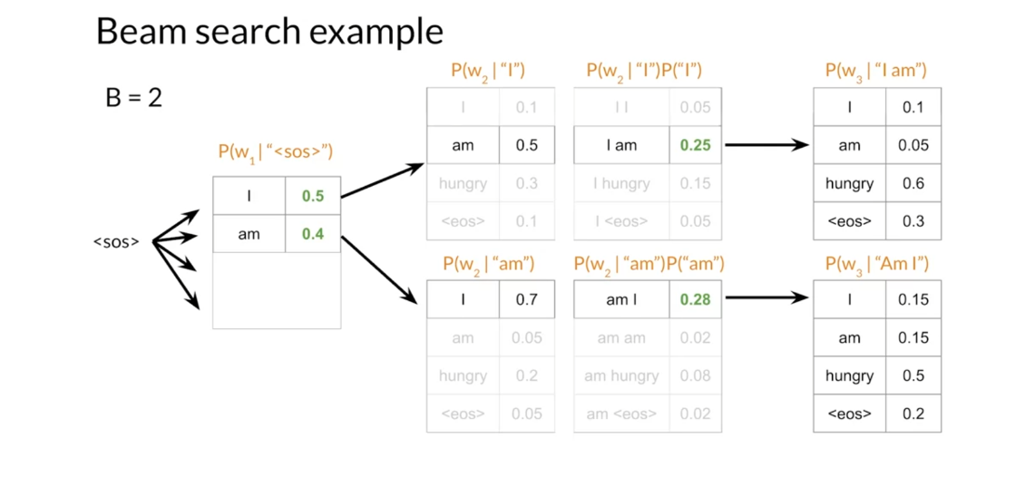
To get the conditional probabilities at
each step you have to use your model. For now let’s focus on the decoder parts
of the model ignoring the encoder and attention mechanism. At the start of the sequence
you will use your decoder to as a vector of probabilities for
each of the words and the vocabulary. This is equivalent to computing
the conditional probability of every word given
the start of sequence token. Then you select the most probable
B outputs from the model and discard all other possibilities. After that you use your model B times to
find the conditional probabilities of all the words in the vocabulary
given the sequences that you kept in the previous step. Then you compute the sequence probability
and keep the B most probable sequences. And you keep doing this until the B
most probable sequences gets to the end of the sequence token. Notes that at each step after
the one where your sequence is only composed by the SOS token you
have to run your model B times.
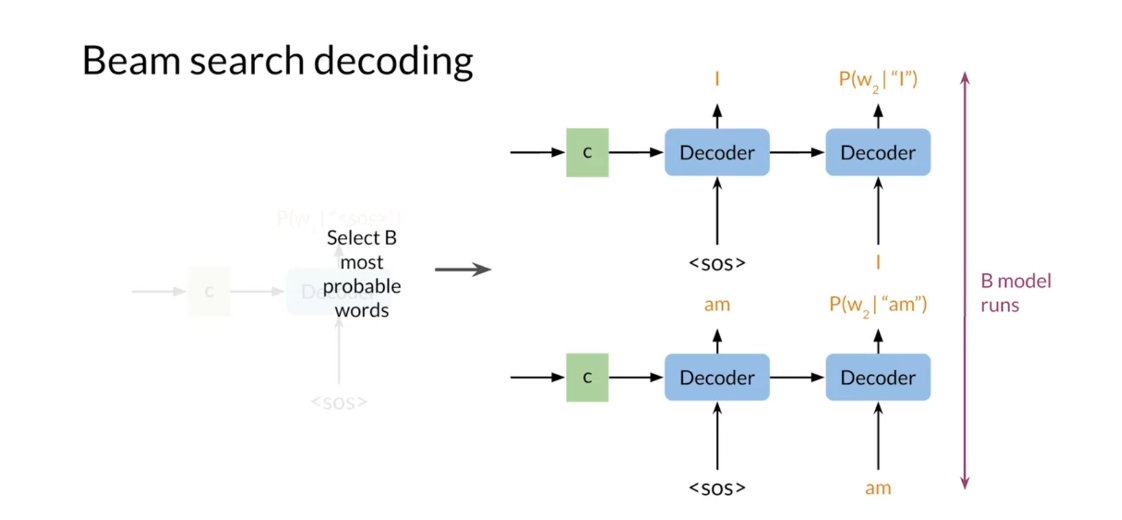
The vanilla version of beam
search has some disadvantages. For instance, it penalizes the choice of long wear
sequences because the probability of a sequence is computed as the product
of multiple conditional probabilities. However, you could normalize the
probability of each sequence by its number four is to avoid this problem. Beam search also requires you to store
the b most probable sequences and computes conditional probabilities
given all of those sequences. Therefore, this method could be
computationally expensive and consumes lots of memory. You have a new tool that you can add to
your toolkit beam search has been widely used for quiet a period of time and
is still used a lot. In the next video, I will show you
another technique that you can use, known as NBR, or minimum based risk.
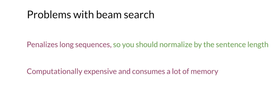
Beam Search(束搜索)是一种用于在生成式模型(如机器翻译、语言模型等)中寻找最优输出序列的搜索算法。它通过在每个时间步保留概率最高的 k 个候选项(称为束宽或束大小),并在下一个时间步基于这些候选项继续扩展搜索,最终找到整个输出序列的最优解。
Beam Search 的工作方式如下:
- 初始化:从起始状态开始,将初始概率分数设置为 1.0,将初始序列设置为空序列。
- 生成候选项:在每个时间步,对于当前所有的候选项,根据模型生成下一个词的概率分布,并选择概率最高的 k 个词作为下一步的候选项。
- 更新概率分数:对于每个候选项,将当前概率分数乘以下一个词的概率得到新的概率分数。
- 剪枝:保留概率分数最高的 k 个候选项,并丢弃其他候选项。
- 终止条件:当生成的序列达到最大长度或者所有候选项均为终止符号时,停止搜索。
- 回溯:从最终的候选项中选择概率最高的序列作为最终输出序列。
Beam Search 的优点是可以在一定程度上减少搜索空间,加快搜索速度,并且能够找到相对较好的解。然而,由于束宽的限制,Beam Search 可能会导致局部最优解,而无法找到全局最优解。因此,在一些情况下,Beam Search 可能需要结合其他技术(如长度惩罚、重复惩罚等)来改善搜索结果。
Minimum Bayes Risk
This is the last technique I will show
you to evaluate your NMT systems. It is very simple and works surprisingly well when compared to
the other techniques, let’s get started. >> Earlier, you encountered random
sampling to choose a probable token and the issues with that decoding method. But if you go a little further with that,
say by generating 30 samples and comparing them all against one another. You’ll see quite a bit of
improvements in your decoding. You’ll have to compare multiple
candidate translations for the minimum bayes risk decoding method,
MBR for shorts. Implementing MBR is
pretty straightforward. Begin by generating several random
samples, then compare each sample against each other using a similarity
score or a loss function. ROUGE would be a good choice that
you may recall from a bit earlier. Finally, choose the sample with
the highest average similarity or the lowest loss.
The translation that you get using this
method is the closest to all candidate translations. This process can be viewed
as some authors suggest, as finding a consensus between
all candidate translations.
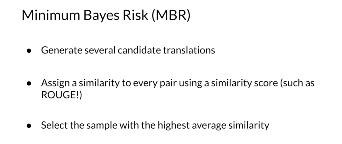
If you decide to use ROUGE score
as a similarity metric for comparing every pair of
candidate translations, you would have MBR summarized
in the formula presented here. Your goal is to find the candidate
translation E that maximizes the average ROUGE score with
every other candidates E prime. So MBR is relatively easy to implement. You need to have multiple
candidate translations and select a way to compare them.
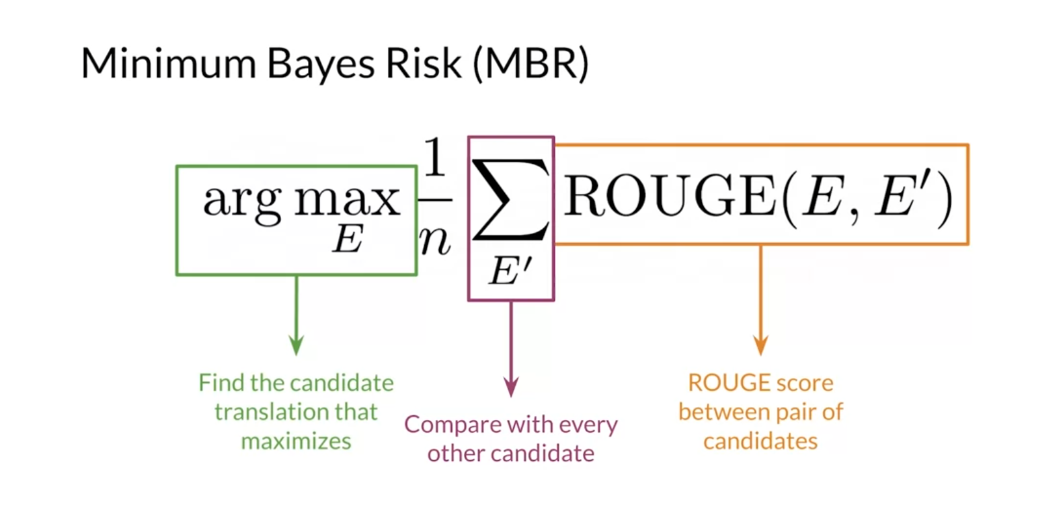
But for the sake of clarity, let’s go through an implementation
process in more detail. Here are the steps for implementing MVR with ROUGE on a small
set of four candidate translations. First, calculate the ROUGE score
between the first C subscript 1 and the second C subscript 2
candidate translations. For the 1st and 3rd and
for the 1st and 4th, then compute the average R subscript
1 using those three rules scores. Then you repeat this process for the other three candidates in your sets to
average ROUGE scores for each one of them. Finally, you select the candidate with
the highest average ROUGE score and that’s it for MBR, you’ll be implementing this method in the
assignment along with a greedy decoder.
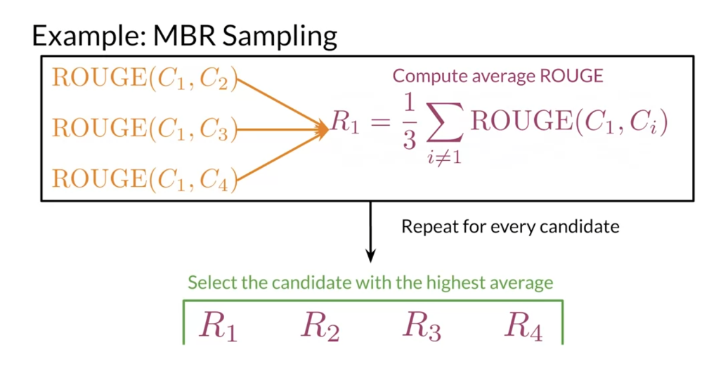
In summary, MBR takes several
translation candidates and compares them against each other. Then chooses the one with the highest
average similarity as the beam search case. This method can give you a more
contextually accurate translation than random sampling and greedy decoding. >> Congratulations on finishing this week,
you now know how to implement in your own machine translation system and
you also know how to evaluate it. Next week, I’ll talk about one of
the states of the arts models known as the transformer, which also makes use
of an encoder decoder architecture.
Quiz

第一题改正:

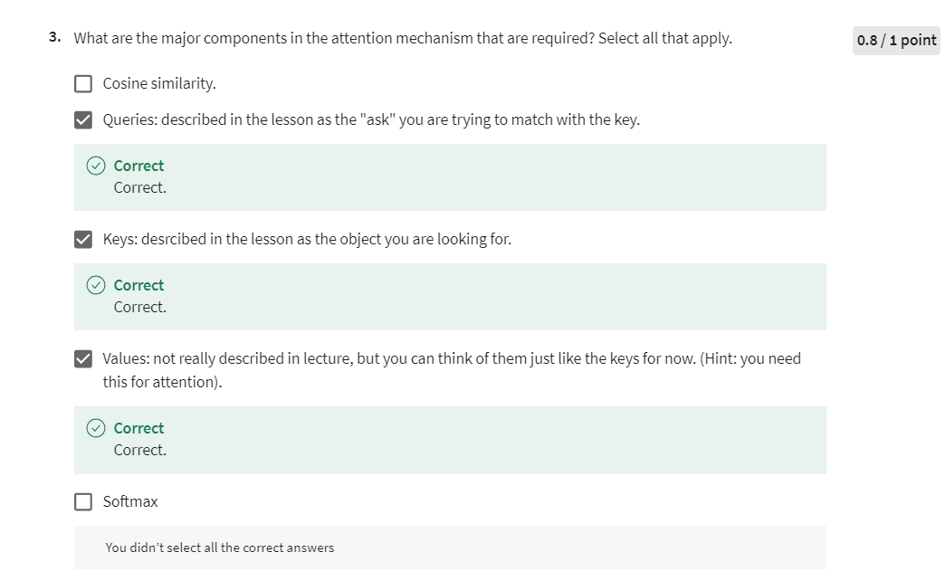
第三题错误示例:第三题正确答案是Keys, Values, Queries, Softmax

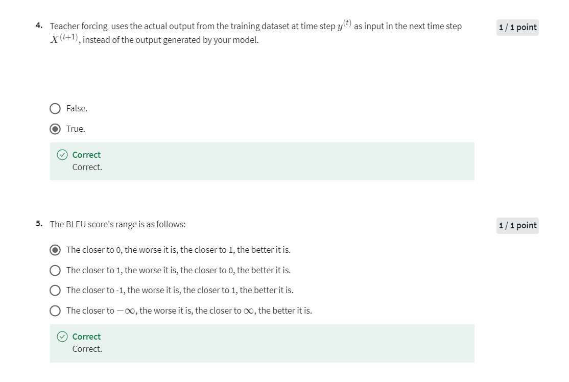
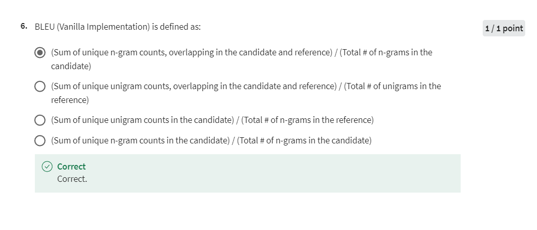

Precision is defined as:
(Sum of overlapping unigrams in model and reference)/(total # of words in model)
Recall is defined as:
(Sum of overlapping unigrams in model and reference)/(total # of words in reference)
In ROUGE, precision measures how many of the words in the generated summary are also present in the reference summary, while recall measures how many of the words in the reference summary are also present in the generated summary.
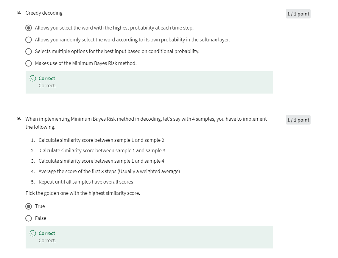
Programming Assignment: NMT with Attention (Tensorflow)
Assignment 1: Neural Machine Translation
Welcome to the first assignment of Course 4. Here, you will build an English-to-Portuguese neural machine translation (NMT) model using Long Short-Term Memory (LSTM) networks with attention. Machine translation is an important task in natural language processing and could be useful not only for translating one language to another but also for word sense disambiguation (e.g. determining whether the word “bank” refers to the financial bank, or the land alongside a river). Implementing this using just a Recurrent Neural Network (RNN) with LSTMs can work for short to medium length sentences but can result in vanishing gradients for very long sequences. To help with this, you will be adding an attention mechanism to allow the decoder to access all relevant parts of the input sentence regardless of its length. By completing this assignment, you will:
- Implement an encoder-decoder system with attention
- Build the NMT model from scratch using Tensorflow
- Generate translations using greedy and Minimum Bayes Risk (MBR) decoding
import os
os.environ['TF_CPP_MIN_LOG_LEVEL'] = '3' # Setting this env variable prevents TF warnings from showing up

import numpy as np
import tensorflow as tf
from collections import Counter
from utils import (sentences, train_data, val_data, english_vectorizer, portuguese_vectorizer,
                   masked_loss, masked_acc, tokens_to_text)

import w1_unittest
utils.py文件如下:
import numpy as np
import tensorflow as tf
import tensorflow_text as tf_text
import pathlib

path_to_file = pathlib.Path("por-eng/por.txt")

np.random.seed(1234)
tf.random.set_seed(1234)

def load_data(path):
    text = path.read_text(encoding="utf-8")

    lines = text.splitlines()
    pairs = [line.split("\t") for line in lines]

    context = np.array([context for target, context, _ in pairs])
    target = np.array([target for target, context, _ in pairs])

    return context, target


portuguese_sentences, english_sentences = load_data(path_to_file)

sentences = (portuguese_sentences, english_sentences)

BUFFER_SIZE = len(english_sentences)
BATCH_SIZE = 64

is_train = np.random.uniform(size=(len(portuguese_sentences),)) < 0.8

train_raw = (
    tf.data.Dataset.from_tensor_slices(
        (english_sentences[is_train], portuguese_sentences[is_train])
    )
    .shuffle(BUFFER_SIZE)
    .batch(BATCH_SIZE)
)
val_raw = (
    tf.data.Dataset.from_tensor_slices(
        (english_sentences[~is_train], portuguese_sentences[~is_train])
    )
    .shuffle(BUFFER_SIZE)
    .batch(BATCH_SIZE)
)


def tf_lower_and_split_punct(text):
    text = tf_text.normalize_utf8(text, "NFKD")
    text = tf.strings.lower(text)
    text = tf.strings.regex_replace(text, "[^ a-z.?!,¿]", "")
    text = tf.strings.regex_replace(text, "[.?!,¿]", r" \0 ")
    text = tf.strings.strip(text)
    text = tf.strings.join(["[SOS]", text, "[EOS]"], separator=" ")
    return text


max_vocab_size = 12000

english_vectorizer = tf.keras.layers.TextVectorization(
    standardize=tf_lower_and_split_punct, max_tokens=max_vocab_size, ragged=True
)

english_vectorizer.adapt(train_raw.map(lambda context, target: context))

portuguese_vectorizer = tf.keras.layers.TextVectorization(
    standardize=tf_lower_and_split_punct, max_tokens=max_vocab_size, ragged=True
)

portuguese_vectorizer.adapt(train_raw.map(lambda context, target: target))


def process_text(context, target):
    context = english_vectorizer(context).to_tensor()
    target = portuguese_vectorizer(target)
    targ_in = target[:, :-1].to_tensor()
    targ_out = target[:, 1:].to_tensor()
    return (context, targ_in), targ_out


train_data = train_raw.map(process_text, tf.data.AUTOTUNE)
val_data = val_raw.map(process_text, tf.data.AUTOTUNE)

del train_raw
del val_raw


def masked_loss(y_true, y_pred):

    loss_fn = tf.keras.losses.SparseCategoricalCrossentropy(from_logits=True, reduction='none')
    loss = loss_fn(y_true, y_pred)

    # Check which elements of y_true are padding
    mask = tf.cast(y_true != 0, loss.dtype)

    loss *= mask
    # Return the total.
    return tf.reduce_sum(loss)/tf.reduce_sum(mask)


def masked_acc(y_true, y_pred):
    y_pred = tf.argmax(y_pred, axis=-1)
    y_pred = tf.cast(y_pred, y_true.dtype)
    match = tf.cast(y_true == y_pred, tf.float32)
    mask = tf.cast(y_true != 0, tf.float32)

    return tf.reduce_sum(match)/tf.reduce_sum(mask)


def tokens_to_text(tokens, id_to_word):
    words = id_to_word(tokens)
    result = tf.strings.reduce_join(words, axis=-1, separator=" ")
    return result
1. Data Preparation
The text pre-processing bits have already been taken care of (if you are interested in this be sure to check the utils.py file). The steps performed can be summarized as:
- Reading the raw data from the text files
- Cleaning the data (using lowercase, adding space around punctuation, trimming whitespaces, etc)
- Splitting it into training and validation sets
- Adding the start-of-sentence and end-of-sentence tokens to every sentence
- Tokenizing the sentences
- Creating a Tensorflow dataset out of the tokenized sentences
Take a moment to inspect the raw sentences:
portuguese_sentences, english_sentences = sentences

print(f"English (to translate) sentence:\n\n{english_sentences[-5]}\n")
print(f"Portuguese (translation) sentence:\n\n{portuguese_sentences[-5]}")
Output
English (to translate) sentence:

No matter how much you try to convince people that chocolate is vanilla, it'll still be chocolate, even though you may manage to convince yourself and a few others that it's vanilla.

Portuguese (translation) sentence:

Não importa o quanto você tenta convencer os outros de que chocolate é baunilha, ele ainda será chocolate, mesmo que você possa convencer a si mesmo e poucos outros de que é baunilha.
You don’t have much use for the raw sentences so delete them to save memory:
del portuguese_sentences
del english_sentences
del sentences
Notice that you imported an english_vectorizer and a portuguese_vectorizer from utils.py. These were created using tf.keras.layers.TextVectorization and they provide interesting features such as ways to visualize the vocabulary and convert text into tokenized ids and vice versa. In fact, you can inspect the first ten words of the vocabularies for both languages:
print(f"First 10 words of the english vocabulary:\n\n{english_vectorizer.get_vocabulary()[:10]}\n")
print(f"First 10 words of the portuguese vocabulary:\n\n{portuguese_vectorizer.get_vocabulary()[:10]}")
Output
First 10 words of the english vocabulary:

['', '[UNK]', '[SOS]', '[EOS]', '.', 'tom', 'i', 'to', 'you', 'the']

First 10 words of the portuguese vocabulary:

['', '[UNK]', '[SOS]', '[EOS]', '.', 'tom', 'que', 'o', 'nao', 'eu']
Notice that the first 4 words are reserved for special words. In order, these are:
- the empty string
- a special token to represent an unknown word
- a special token to represent the start of a sentence
- a special token to represent the end of a sentence
You can see how many words are in a vocabulary by using the vocabulary_size method:
# Size of the vocabulary
vocab_size_por = portuguese_vectorizer.vocabulary_size()
vocab_size_eng = english_vectorizer.vocabulary_size()

print(f"Portuguese vocabulary is made up of {vocab_size_por} words")
print(f"English vocabulary is made up of {vocab_size_eng} words")
Output
Portuguese vocabulary is made up of 12000 words
English vocabulary is made up of 12000 words
You can define tf.keras.layers.StringLookup objects that will help you map from words to ids and vice versa. Do this for the portuguese vocabulary since this will be useful later on when you decode the predictions from your model:
# This helps you convert from words to ids
word_to_id = tf.keras.layers.StringLookup(
    vocabulary=portuguese_vectorizer.get_vocabulary(),
    mask_token="",
    oov_token="[UNK]"
)

# This helps you convert from ids to words
id_to_word = tf.keras.layers.StringLookup(
    vocabulary=portuguese_vectorizer.get_vocabulary(),
    mask_token="",
    oov_token="[UNK]",
    invert=True,
)
Try it out for the special tokens and a random word:
unk_id = word_to_id("[UNK]")
sos_id = word_to_id("[SOS]")
eos_id = word_to_id("[EOS]")
baunilha_id = word_to_id("baunilha")

print(f"The id for the [UNK] token is {unk_id}")
print(f"The id for the [SOS] token is {sos_id}")
print(f"The id for the [EOS] token is {eos_id}")
print(f"The id for baunilha (vanilla) is {baunilha_id}")
Output
The id for the [UNK] token is 1
The id for the [SOS] token is 2
The id for the [EOS] token is 3
The id for baunilha (vanilla) is 7079
Finally take a look at how the data that is going to be fed to the neural network looks like. Both train_data and val_data are of type tf.data.Dataset and are already arranged in batches of 64 examples. To get the first batch out of a tf dataset you can use the take method. To get the first example out of the batch you can slice the tensor and use the numpy method for nicer printing:
for (to_translate, sr_translation), translation in train_data.take(1):
    print(f"Tokenized english sentence:\n{to_translate[0, :].numpy()}\n\n")
    print(f"Tokenized portuguese sentence (shifted to the right):\n{sr_translation[0, :].numpy()}\n\n")
    print(f"Tokenized portuguese sentence:\n{translation[0, :].numpy()}\n\n")
Output
Tokenized english sentence:
[   2  210    9  146  123   38    9 1672    4    3    0    0    0    0]


Tokenized portuguese sentence (shifted to the right):
[   2 1085    7  128   11  389   37 2038    4    0    0    0    0    0
    0]


Tokenized portuguese sentence:
[1085    7  128   11  389   37 2038    4    3    0    0    0    0    0
    0]
There are a couple of important details to notice.
- Padding has already been applied to the tensors and the value used for this is 0
- Each example consists of 3 different tensors:
- The sentence to translate
- The shifted-to-the-right translation
- The translation
The first two can be considered as the features, while the third one as the target. By doing this your model can perform Teacher Forcing as you saw in the lectures.
Now it is time to begin coding!
2. NMT model with attention
The model you will build uses an encoder-decoder architecture. This Recurrent Neural Network (RNN) takes in a tokenized version of a sentence in its encoder, then passes it on to the decoder for translation. As mentioned in the lectures, just using a a regular sequence-to-sequence model with LSTMs will work effectively for short to medium sentences but will start to degrade for longer ones. You can picture it like the figure below where all of the context of the input sentence is compressed into one vector that is passed into the decoder block. You can see how this will be an issue for very long sentences (e.g. 100 tokens or more) because the context of the first parts of the input will have very little effect on the final vector passed to the decoder.

Adding an attention layer to this model avoids this problem by giving the decoder access to all parts of the input sentence. To illustrate, let’s just use a 4-word input sentence as shown below. Remember that a hidden state is produced at each timestep of the encoder (represented by the orange rectangles). These are all passed to the attention layer and each are given a score given the current activation (i.e. hidden state) of the decoder. For instance, let’s consider the figure below where the first prediction “como” is already made. To produce the next prediction, the attention layer will first receive all the encoder hidden states (i.e. orange rectangles) as well as the decoder hidden state when producing the word “como” (i.e. first green rectangle). Given this information, it will score each of the encoder hidden states to know which one the decoder should focus on to produce the next word. As a result of training, the model might have learned that it should align to the second encoder hidden state and subsequently assigns a high probability to the word “você”. If we are using greedy decoding, we will output the said word as the next symbol, then restart the process to produce the next word until we reach an end-of-sentence prediction.
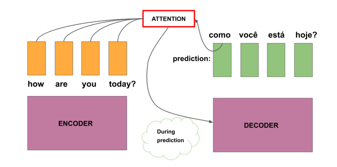
There are different ways to implement attention and the one we’ll use for this assignment is the Scaled Dot Product Attention which has the form:
A t t e n t i o n ( Q , K , V ) = s o f t m a x ( Q K T d k ) V Attention(Q, K, V) = softmax(\frac{QK^T}{\sqrt{d_k}})V Attention(Q,K,V)=softmax(dkQKT)V
You will dive deeper into this equation in the next week but for now, you can think of it as computing scores using queries (Q) and keys (K), followed by a multiplication of values (V) to get a context vector at a particular timestep of the decoder. This context vector is fed to the decoder RNN to get a set of probabilities for the next predicted word. The division by square root of the keys dimensionality ( d k \sqrt{d_k} dk) is for improving model performance and you’ll also learn more about it next week. For our machine translation application, the encoder activations (i.e. encoder hidden states) will be the keys and values, while the decoder activations (i.e. decoder hidden states) will be the queries.
You will see in the upcoming sections that this complex architecture and mechanism can be implemented with just a few lines of code.
First you will define two important global variables:
- The size of the vocabulary
- The number of units in the LSTM layers (the same number will be used for all LSTM layers)
In this assignment, the vocabulary sizes for English and Portuguese are the same. Therefore, we use a single constant VOCAB_SIZE throughout the notebook. While in other settings, vocabulary sizes could differ, that is not the case in our assignment.
VOCAB_SIZE = 12000
UNITS = 256
Exercise 1 - Encoder
Your first exercise is to code the encoder part of the neural network. For this, complete the Encoder class below. Notice that in the constructor (the __init__ method) you need to define all of the sublayers of the encoder and then use these sublayers during the forward pass (the call method).
The encoder consists of the following layers:
- Embedding. For this layer you need to define the appropriate
input_dimandoutput_dimand let it know that you are using ‘0’ as padding, which can be done by using the appropriate value for themask_zeroparameter.
- Bidirectional LSTM. In TF you can implement bidirectional behaviour for RNN-like layers. This part is already taken care of but you will need to specify the appropriate type of layer as well as its parameters. In particular you need to set the appropriate number of units and make sure that the LSTM returns the full sequence and not only the last output, which can be done by using the appropriate value for the
return_sequencesparameter.
You need to define the forward pass using the syntax of TF’s functional API. What this means is that you chain function calls together to define your network like this:
encoder_input = keras.Input(shape=(28, 28, 1), name="original_img")
x = layers.Conv2D(16, 3, activation="relu")(encoder_input)
x = layers.MaxPooling2D(3)(x)
x = layers.Conv2D(16, 3, activation="relu")(x)
encoder_output = layers.GlobalMaxPooling2D()(x)
# GRADED CLASS: Encoder
class Encoder(tf.keras.layers.Layer):
    def __init__(self, vocab_size, units):
        """Initializes an instance of this class

        Args:
            vocab_size (int): Size of the vocabulary
            units (int): Number of units in the LSTM layer
        """
        super(Encoder, self).__init__()

        ### START CODE HERE ###

        self.embedding = tf.keras.layers.Embedding(
            input_dim=vocab_size,
            output_dim=units,
            mask_zero=True
        )

        self.rnn = tf.keras.layers.Bidirectional(
            merge_mode="sum",
            layer=tf.keras.layers.LSTM(
                units=units,
                return_sequences=True
            ),
        )

        ### END CODE HERE ###

    def call(self, context):
        """Forward pass of this layer

        Args:
            context (tf.Tensor): The sentence to translate

        Returns:
            tf.Tensor: Encoded sentence to translate
        """

        ### START CODE HERE ###

        # Pass the context through the embedding layer
        x = self.embedding(context)

        # Pass the output of the embedding through the RNN
        x = self.rnn(x)

        ### END CODE HERE ###

        return x
# Do a quick check of your implementation

# Create an instance of your class
encoder = Encoder(VOCAB_SIZE, UNITS)

# Pass a batch of sentences to translate from english to portuguese
encoder_output = encoder(to_translate)

print(f'Tensor of sentences in english has shape: {to_translate.shape}\n')
print(f'Encoder output has shape: {encoder_output.shape}')
Output
Tensor of sentences in english has shape: (64, 14)

Encoder output has shape: (64, 14, 256)
Expected Output
Tensor of sentences in english has shape: (64, 14)

Encoder output has shape: (64, 14, 256)
# Test your code!

w1_unittest.test_encoder(Encoder)
Output
All tests passed!
Exercise 2 - CrossAttention
Your next exercise is to code the layer that will perform cross attention between the original sentences and the translations. For this, complete the CrossAttention class below. Notice that in the constructor (the __init__ method) you need to define all of the sublayers and then use these sublayers during the forward pass (the call method). For this particular case some of these bits are already taken care of.
The cross attention consists of the following layers:
- MultiHeadAttention. For this layer you need to define the appropriate
key_dim, which is the size of the key and query tensors. You will also need to set the number of heads to 1 since you aren’t implementing multi head attention but attention between two tensors. The reason why this layer is preferred over Attention is that it allows simpler code during the forward pass.
A couple of things to notice:
- You need a way to pass both the output of the attention alongside the shifted-to-the-right translation (since this cross attention happens in the decoder side). For this you will use an Add layer so that the original dimension is preserved, which would not happen if you use something like a Concatenate layer.
- Layer normalization is also performed for better stability of the network by using a LayerNormalization layer.
- You don’t need to worry about these last steps as these are already solved.
# GRADED CLASS: CrossAttention
class CrossAttention(tf.keras.layers.Layer):
    def __init__(self, units):
        """Initializes an instance of this class

        Args:
            units (int): Number of units in the LSTM layer
        """
        super().__init__()

        ### START CODE HERE ###

        self.mha = (
            tf.keras.layers.MultiHeadAttention(
                key_dim=units,
                num_heads=1
            )
        )

        ### END CODE HERE ###

        self.layernorm = tf.keras.layers.LayerNormalization()
        self.add = tf.keras.layers.Add()

    def call(self, context, target):
        """Forward pass of this layer

        Args:
            context (tf.Tensor): Encoded sentence to translate
            target (tf.Tensor): The embedded shifted-to-the-right translation

        Returns:
            tf.Tensor: Cross attention between context and target
        """
        ### START CODE HERE ###

        # Call the MH attention by passing in the query and value
        # For this case the query should be the translation and the value the encoded sentence to translate
        # Hint: Check the call arguments of MultiHeadAttention in the docs
        attn_output = self.mha(
            query=target,
            value=context
        )

        ### END CODE HERE ###

        x = self.add([target, attn_output])

        x = self.layernorm(x)

        return x
# Do a quick check of your implementation

# Create an instance of your class
attention_layer = CrossAttention(UNITS)

# The attention layer expects the embedded sr-translation and the context
# The context (encoder_output) is already embedded so you need to do this for sr_translation:
sr_translation_embed = tf.keras.layers.Embedding(VOCAB_SIZE, output_dim=UNITS, mask_zero=True)(sr_translation)

# Compute the cross attention
attention_result = attention_layer(encoder_output, sr_translation_embed)

print(f'Tensor of contexts has shape: {encoder_output.shape}')
print(f'Tensor of translations has shape: {sr_translation_embed.shape}')
print(f'Tensor of attention scores has shape: {attention_result.shape}')
Output
Tensor of contexts has shape: (64, 14, 256)
Tensor of translations has shape: (64, 15, 256)
Tensor of attention scores has shape: (64, 15, 256)
Expected Output
Tensor of contexts has shape: (64, 14, 256)
Tensor of translations has shape: (64, 15, 256)
Tensor of attention scores has shape: (64, 15, 256)
# Test your code!

w1_unittest.test_cross_attention(CrossAttention)
Output
All tests passed!
Exercise 3 - Decoder
Now you will implement the decoder part of the neural network by completing the Decoder class below. Notice that in the constructor (the __init__ method) you need to define all of the sublayers of the decoder and then use these sublayers during the forward pass (the call method).
The decoder consists of the following layers:
- Embedding. For this layer you need to define the appropriate
input_dimandoutput_dimand let it know that you are using ‘0’ as padding, which can be done by using the appropriate value for themask_zeroparameter.
- Pre-attention LSTM. Unlike in the encoder in which you used a Bidirectional LSTM, here you will use a vanilla LSTM. Don’t forget to set the appropriate number of units and make sure that the LSTM returns the full sequence and not only the last output, which can be done by using the appropriate value for the
return_sequencesparameter. It is very important that this layer returns the state since this will be needed for inference so make sure to set thereturn_stateparameter accordingly. Notice that LSTM layers return state as a tuple of two tensors calledmemory_stateandcarry_state, however these names have been changed to better reflect what you have seen in the lectures tohidden_stateandcell_staterespectively.
- The attention layer that performs cross attention between the sentence to translate and the right-shifted translation. Here you need to use the
CrossAttentionlayer you defined in the previous exercise.
- Post-attention LSTM. Another LSTM layer. For this one you don’t need it to return the state.
- Finally a Dense layer. This one should have the same number of units as the size of the vocabulary since you expect it to compute the logits for every possible word in the vocabulary. Make sure to use a
logsoftmaxactivation function for this one, which you can get as tf.nn.log_softmax.
# GRADED CLASS: Decoder
class Decoder(tf.keras.layers.Layer):
    def __init__(self, vocab_size, units):
        """Initializes an instance of this class

        Args:
            vocab_size (int): Size of the vocabulary
            units (int): Number of units in the LSTM layer
        """
        super(Decoder, self).__init__()

        ### START CODE HERE ###

        # The embedding layer
        self.embedding = tf.keras.layers.Embedding(
            input_dim=vocab_size,
            output_dim=units,
            mask_zero=True
        )

        # The RNN before attention
        self.pre_attention_rnn = tf.keras.layers.LSTM(
            units=units,
            return_sequences=True,
            return_state=True
        )

        # The attention layer
        self.attention = CrossAttention(units)

        # The RNN after attention
        self.post_attention_rnn = tf.keras.layers.LSTM(
            units=units,
            return_sequences=True
        )

        # The dense layer with logsoftmax activation
        self.output_layer = tf.keras.layers.Dense(
            units=vocab_size,
            activation=tf.nn.log_softmax
        )

        ### END CODE HERE ###

    def call(self, context, target, state=None, return_state=False):
        """Forward pass of this layer

        Args:
            context (tf.Tensor): Encoded sentence to translate
            target (tf.Tensor): The shifted-to-the-right translation
            state (list[tf.Tensor, tf.Tensor], optional): Hidden state of the pre-attention LSTM. Defaults to None.
            return_state (bool, optional): If set to true return the hidden states of the LSTM. Defaults to False.

        Returns:
            tf.Tensor: The log_softmax probabilities of predicting a particular token
        """
        ### START CODE HERE ###

        # Get the embedding of the input
        x = self.embedding(target)

        # Pass the embedded input into the pre attention LSTM
        # Hints:
        # - The LSTM you defined earlier should return the output alongside the state (made up of two tensors)
        # - Pass in the state to the LSTM (needed for inference)
        x, hidden_state, cell_state = self.pre_attention_rnn(x, initial_state=state)

        # Perform cross attention between the context and the output of the LSTM (in that order)
        x = self.attention(context, x)

        # Do a pass through the post attention LSTM
        x = self.post_attention_rnn(x)

        # Compute the logits
        logits = self.output_layer(x)

        ### END CODE HERE ###

        if return_state:
            return logits, [hidden_state, cell_state]

        return logits
# Do a quick check of your implementation

# Create an instance of your class
decoder = Decoder(VOCAB_SIZE, UNITS)

# Notice that you don't need the embedded version of sr_translation since this is done inside the class
logits = decoder(encoder_output, sr_translation)

print(f'Tensor of contexts has shape: {encoder_output.shape}')
print(f'Tensor of right-shifted translations has shape: {sr_translation.shape}')
print(f'Tensor of logits has shape: {logits.shape}')
Output
Tensor of contexts has shape: (64, 14, 256)
Tensor of right-shifted translations has shape: (64, 15)
Tensor of logits has shape: (64, 15, 12000)
Expected Output
Tensor of contexts has shape: (64, 14, 256)
Tensor of right-shifted translations has shape: (64, 15)
Tensor of logits has shape: (64, 15, 12000)
# Test your code!

w1_unittest.test_decoder(Decoder, CrossAttention)
Output
All tests passed!
Exercise 4 - Translator
Now you have to put together all of the layers you previously coded into an actual model. For this, complete the Translator class below. Notice how unlike the Encoder and Decoder classes inherited from tf.keras.layers.Layer, the Translator class inherits from tf.keras.Model.
Remember that train_data will yield a tuple with the sentence to translate and the shifted-to-the-right translation, which are the “features” of the model. This means that the inputs of your network will be tuples containing context and targets.
# GRADED CLASS: Translator
class Translator(tf.keras.Model):
    def __init__(self, vocab_size, units):
        """Initializes an instance of this class

        Args:
            vocab_size (int): Size of the vocabulary
            units (int): Number of units in the LSTM layer
        """
        super().__init__()

        ### START CODE HERE ###

        # Define the encoder with the appropriate vocab_size and number of units
        self.encoder = Encoder(vocab_size, units)

        # Define the decoder with the appropriate vocab_size and number of units
        self.decoder = Decoder(vocab_size, units)

        ### END CODE HERE ###

    def call(self, inputs):
        """Forward pass of this layer

        Args:
            inputs (tuple(tf.Tensor, tf.Tensor)): Tuple containing the context (sentence to translate) and the target (shifted-to-the-right translation)

        Returns:
            tf.Tensor: The log_softmax probabilities of predicting a particular token
        """

        ### START CODE HERE ###

        # In this case inputs is a tuple consisting of the context and the target, unpack it into single variables
        context, target = inputs

        # Pass the context through the encoder
        encoded_context = self.encoder(context)

        # Compute the logits by passing the encoded context and the target to the decoder
        logits = self.decoder(encoded_context, target)

        ### END CODE HERE ###

        return logits
# Do a quick check of your implementation

# Create an instance of your class
translator = Translator(VOCAB_SIZE, UNITS)

# Compute the logits for every word in the vocabulary
logits = translator((to_translate, sr_translation))

print(f'Tensor of sentences to translate has shape: {to_translate.shape}')
print(f'Tensor of right-shifted translations has shape: {sr_translation.shape}')
print(f'Tensor of logits has shape: {logits.shape}')
Output
Tensor of sentences to translate has shape: (64, 14)
Tensor of right-shifted translations has shape: (64, 15)
Tensor of logits has shape: (64, 15, 12000)
Expected Output
Tensor of sentences to translate has shape: (64, 14)
Tensor of right-shifted translations has shape: (64, 15)
Tensor of logits has shape: (64, 15, 12000)
w1_unittest.test_translator(Translator, Encoder, Decoder)
Output
All tests passed!
3. Training
Now that you have an untrained instance of the NMT model, it is time to train it. You can use the compile_and_train function below to achieve this:
def compile_and_train(model, epochs=20, steps_per_epoch=500):
    model.compile(optimizer="adam", loss=masked_loss, metrics=[masked_acc, masked_loss])

    history = model.fit(
        train_data.repeat(),
        epochs=epochs,
        steps_per_epoch=steps_per_epoch,
        validation_data=val_data,
        validation_steps=50,
        callbacks=[tf.keras.callbacks.EarlyStopping(patience=3)],
    )

    return model, history
# Train the translator (this takes some minutes so feel free to take a break)

trained_translator, history = compile_and_train(translator)
Output
Epoch 1/20
500/500 [==============================] - 48s 68ms/step - loss: 5.1397 - masked_acc: 0.2225 - masked_loss: 5.1422 - val_loss: 4.2776 - val_masked_acc: 0.3481 - val_masked_loss: 4.2784
Epoch 2/20
500/500 [==============================] - 16s 33ms/step - loss: 3.6741 - masked_acc: 0.4191 - masked_loss: 3.6749 - val_loss: 3.0218 - val_masked_acc: 0.4965 - val_masked_loss: 3.0237
Epoch 3/20
500/500 [==============================] - 16s 32ms/step - loss: 2.7304 - masked_acc: 0.5441 - masked_loss: 2.7319 - val_loss: 2.3823 - val_masked_acc: 0.5844 - val_masked_loss: 2.3826
Epoch 4/20
500/500 [==============================] - 16s 32ms/step - loss: 2.2110 - masked_acc: 0.6180 - masked_loss: 2.2119 - val_loss: 1.9733 - val_masked_acc: 0.6483 - val_masked_loss: 1.9741
Epoch 5/20
500/500 [==============================] - 16s 31ms/step - loss: 1.8569 - masked_acc: 0.6690 - masked_loss: 1.8581 - val_loss: 1.7101 - val_masked_acc: 0.6829 - val_masked_loss: 1.7105
Epoch 6/20
500/500 [==============================] - 15s 30ms/step - loss: 1.5978 - masked_acc: 0.7010 - masked_loss: 1.5987 - val_loss: 1.5794 - val_masked_acc: 0.7062 - val_masked_loss: 1.5785
Epoch 7/20
500/500 [==============================] - 15s 31ms/step - loss: 1.4876 - masked_acc: 0.7169 - masked_loss: 1.4883 - val_loss: 1.4743 - val_masked_acc: 0.7138 - val_masked_loss: 1.4749
Epoch 8/20
500/500 [==============================] - 16s 32ms/step - loss: 1.3877 - masked_acc: 0.7300 - masked_loss: 1.3886 - val_loss: 1.3770 - val_masked_acc: 0.7270 - val_masked_loss: 1.3786
Epoch 9/20
500/500 [==============================] - 16s 32ms/step - loss: 1.3113 - masked_acc: 0.7391 - masked_loss: 1.3126 - val_loss: 1.2842 - val_masked_acc: 0.7379 - val_masked_loss: 1.2841
Epoch 10/20
500/500 [==============================] - 16s 31ms/step - loss: 1.1826 - masked_acc: 0.7548 - masked_loss: 1.1840 - val_loss: 1.2217 - val_masked_acc: 0.7491 - val_masked_loss: 1.2225
Epoch 11/20
500/500 [==============================] - 15s 30ms/step - loss: 1.0788 - masked_acc: 0.7676 - masked_loss: 1.0797 - val_loss: 1.1737 - val_masked_acc: 0.7615 - val_masked_loss: 1.1739
Epoch 12/20
500/500 [==============================] - 15s 30ms/step - loss: 1.0570 - masked_acc: 0.7716 - masked_loss: 1.0579 - val_loss: 1.1306 - val_masked_acc: 0.7603 - val_masked_loss: 1.1307
Epoch 13/20
500/500 [==============================] - 15s 31ms/step - loss: 1.0358 - masked_acc: 0.7733 - masked_loss: 1.0369 - val_loss: 1.1341 - val_masked_acc: 0.7596 - val_masked_loss: 1.1348
Epoch 14/20
500/500 [==============================] - 15s 31ms/step - loss: 1.0092 - masked_acc: 0.7777 - masked_loss: 1.0103 - val_loss: 1.0890 - val_masked_acc: 0.7683 - val_masked_loss: 1.0894
Epoch 15/20
500/500 [==============================] - 16s 31ms/step - loss: 0.9015 - masked_acc: 0.7928 - masked_loss: 0.9026 - val_loss: 1.0708 - val_masked_acc: 0.7712 - val_masked_loss: 1.0722
Epoch 16/20
500/500 [==============================] - 15s 31ms/step - loss: 0.8550 - masked_acc: 0.7989 - masked_loss: 0.8556 - val_loss: 1.0757 - val_masked_acc: 0.7720 - val_masked_loss: 1.0774
Epoch 17/20
500/500 [==============================] - 15s 31ms/step - loss: 0.8635 - masked_acc: 0.7969 - masked_loss: 0.8643 - val_loss: 1.0103 - val_masked_acc: 0.7784 - val_masked_loss: 1.0115
Epoch 18/20
500/500 [==============================] - 16s 32ms/step - loss: 0.8636 - masked_acc: 0.7970 - masked_loss: 0.8643 - val_loss: 1.0002 - val_masked_acc: 0.7817 - val_masked_loss: 1.0015
Epoch 19/20
500/500 [==============================] - 15s 31ms/step - loss: 0.8465 - masked_acc: 0.7990 - masked_loss: 0.8471 - val_loss: 0.9914 - val_masked_acc: 0.7835 - val_masked_loss: 0.9912
Epoch 20/20
500/500 [==============================] - 16s 31ms/step - loss: 0.7365 - masked_acc: 0.8181 - masked_loss: 0.7373 - val_loss: 0.9863 - val_masked_acc: 0.7834 - val_masked_loss: 0.9869
4. Using the model for inference
Now that your model is trained you can use it for inference. To help you with this the generate_next_token function is provided. Notice that this function is meant to be used inside a for-loop, so you feed to it the information of the previous step to generate the information of the next step. In particular you need to keep track of the state of the pre-attention LSTM in the decoder and if you are done with the translation. Also notice that a temperature variable is introduced which determines how to select the next token given the predicted logits:
def generate_next_token(decoder, context, next_token, done, state, temperature=0.0):
    """Generates the next token in the sequence

    Args:
        decoder (Decoder): The decoder
        context (tf.Tensor): Encoded sentence to translate
        next_token (tf.Tensor): The predicted next token
        done (bool): True if the translation is complete
        state (list[tf.Tensor, tf.Tensor]): Hidden states of the pre-attention LSTM layer
        temperature (float, optional): The temperature that controls the randomness of the predicted tokens. Defaults to 0.0.

    Returns:
        tuple(tf.Tensor, np.float, list[tf.Tensor, tf.Tensor], bool): The next token, log prob of said token, hidden state of LSTM and if translation is done
    """
    # Get the logits and state from the decoder
    logits, state = decoder(context, next_token, state=state, return_state=True)

    # Trim the intermediate dimension
    logits = logits[:, -1, :]

    # If temp is 0 then next_token is the argmax of logits
    if temperature == 0.0:
        next_token = tf.argmax(logits, axis=-1)

    # If temp is not 0 then next_token is sampled out of logits
    else:
        logits = logits / temperature
        next_token = tf.random.categorical(logits, num_samples=1)

    # Trim dimensions of size 1
    logits = tf.squeeze(logits)
    next_token = tf.squeeze(next_token)

    # Get the logit of the selected next_token
    logit = logits[next_token].numpy()

    # Reshape to (1,1) since this is the expected shape for text encoded as TF tensors
    next_token = tf.reshape(next_token, shape=(1,1))

    # If next_token is End-of-Sentence token you are done
    if next_token == eos_id:
        done = True

    return next_token, logit, state, done
See how it works by running the following cell:
# PROCESS SENTENCE TO TRANSLATE AND ENCODE

# A sentence you wish to translate
eng_sentence = "I love languages"

# Convert it to a tensor
texts = tf.convert_to_tensor(eng_sentence)[tf.newaxis]

# Vectorize it and pass it through the encoder
context = english_vectorizer(texts).to_tensor()
context = encoder(context)

# SET STATE OF THE DECODER

# Next token is Start-of-Sentence since you are starting fresh
next_token = tf.fill((1,1), sos_id)

# Hidden and Cell states of the LSTM can be mocked using uniform samples
state = [tf.random.uniform((1, UNITS)), tf.random.uniform((1, UNITS))]

# You are not done until next token is EOS token
done = False

# Generate next token
next_token, logit, state, done = generate_next_token(decoder, context, next_token, done, state, temperature=0.5)
print(f"Next token: {next_token}\nLogit: {logit:.4f}\nDone? {done}")
Output
Next token: [[8841]]
Logit: -18.7456
Done? False
Exercise 5 - translate
Now you can put everything together to translate a given sentence. For this, complete the translate function below. This function will take care of the following steps:
- Process the sentence to translate and encode it
- Set the initial state of the decoder
- Get predictions of the next token (starting with the <SOS> token) for a maximum of iterations (in case the <EOS> token is never returned)
- Return the translated text (as a string), the logit of the last iteration (this helps measure how certain was that the sequence was translated in its totality) and the translation in token format.
Hints:
- The previous cell provides a lot of insights on how this function should work, so if you get stuck refer to it.
Some useful docs:
# GRADED FUNCTION: translate
def translate(model, text, max_length=50, temperature=0.0):
    """Translate a given sentence from English to Portuguese

    Args:
        model (tf.keras.Model): The trained translator
        text (string): The sentence to translate
        max_length (int, optional): The maximum length of the translation. Defaults to 50.
        temperature (float, optional): The temperature that controls the randomness of the predicted tokens. Defaults to 0.0.

    Returns:
        tuple(str, np.float, tf.Tensor): The translation, logit that predicted <EOS> token and the tokenized translation
    """
    # Lists to save tokens and logits
    tokens, logits = [], []

    ### START CODE HERE ###

    # PROCESS THE SENTENCE TO TRANSLATE

    # Convert the original string into a tensor
    text = tf.convert_to_tensor(text)[tf.newaxis]

    # Vectorize the text using the correct vectorizer
    context = english_vectorizer(text).to_tensor()

    # Get the encoded context (pass the context through the encoder)
    # Hint: Remember you can get the encoder by using model.encoder
    context = model.encoder(context)

    # INITIAL STATE OF THE DECODER

    # First token should be SOS token with shape (1,1)
    next_token = tf.fill((1, 1), sos_id)

    # Initial hidden and cell states should be tensors of zeros with shape (1, UNITS)
    state = [tf.zeros((1, UNITS)), tf.zeros((1, UNITS))]

    # You are done when you draw a EOS token as next token (initial state is False)
    done = False

    # Iterate for max_length iterations
    for i in range(max_length):
        # Generate the next token
        try:
            next_token, logit, state, done = generate_next_token(
                decoder=model.decoder,
                context=context,
                next_token=next_token,
                done=done,
                state=state,
                temperature=temperature
            )
        except:
             raise Exception("Problem generating the next token")

        # If done then break out of the loop
        if done:
            break

        # Add next_token to the list of tokens
        tokens.append(next_token)

        # Add logit to the list of logits
        logits.append(logit)

    ### END CODE HERE ###

    # Concatenate all tokens into a tensor
    tokens = tf.concat(tokens, axis=-1)

    # Convert the translated tokens into text
    translation = tf.squeeze(tokens_to_text(tokens, id_to_word))
    translation = translation.numpy().decode()

    return translation, logits[-1], tokens
Try your function with temperature of 0, which will yield a deterministic output and is equivalent to a greedy decoding:
# Running this cell multiple times should return the same output since temp is 0

temp = 0.0
original_sentence = "I love languages"

translation, logit, tokens = translate(trained_translator, original_sentence, temperature=temp)

print(f"Temperature: {temp}\n\nOriginal sentence: {original_sentence}\nTranslation: {translation}\nTranslation tokens:{tokens}\nLogit: {logit:.3f}")
Output
Temperature: 0.0

Original sentence: I love languages
Translation: eu adoro idiomas ja .
Translation tokens:[[  9 564 850  69   4]]
Logit: -1.165
Try your function with temperature of 0.7 (stochastic output):
# Running this cell multiple times should return different outputs since temp is not 0
# You can try different temperatures

temp = 0.7
original_sentence = "I love languages"

translation, logit, tokens = translate(trained_translator, original_sentence, temperature=temp)

print(f"Temperature: {temp}\n\nOriginal sentence: {original_sentence}\nTranslation: {translation}\nTranslation tokens:{tokens}\nLogit: {logit:.3f}")
Output
Temperature: 0.7

Original sentence: I love languages
Translation: eu amo linguas em favor .
Translation tokens:[[   9  522 1032   22   90    4]]
Logit: -1.007
w1_unittest.test_translate(translate, trained_translator)
Output
All tests passed!
5. Minimum Bayes-Risk Decoding
As mentioned in the lectures, getting the most probable token at each step may not necessarily produce the best results. Another approach is to do Minimum Bayes Risk Decoding or MBR. The general steps to implement this are:
- Take several random samples
- Score each sample against all other samples
- Select the one with the highest score
You will be building helper functions for these steps in the following sections.
With the ability to generate different translations by setting different temperature values you can do what you saw in the lectures and generate a bunch of translations and then determine which one is the best candidate. You will now do this by using the provided generate_samples function. This function will return any desired number of candidate translations alongside the log-probability for each one:
def generate_samples(model, text, n_samples=4, temperature=0.6):

    samples, log_probs = [], []

    # Iterate for n_samples iterations
    for _ in range(n_samples):

        # Save the logit and the translated tensor
        _, logp, sample = translate(model, text, temperature=temperature)

        # Save the translated tensors
        samples.append(np.squeeze(sample.numpy()).tolist())

        # Save the logits
        log_probs.append(logp)

    return samples, log_probs
samples, log_probs = generate_samples(trained_translator, 'I love languages')

for s, l in zip(samples, log_probs):
    print(f"Translated tensor: {s} has logit: {l:.3f}")
Output
Translated tensor: [9, 9, 522, 850, 12, 256, 4] has logit: -0.625
Translated tensor: [9, 9, 522, 850, 69, 4] has logit: -1.636
Translated tensor: [9, 564, 850, 38, 8138, 4] has logit: -0.201
Translated tensor: [9, 522, 850, 12, 256, 4] has logit: -0.694
Comparing overlaps
Now that you can generate multiple translations it is time to come up with a method to measure the goodness of each one. As you saw in the lectures, one way to achieve this is by comparing each sample against the others.
There are several metrics you can use for this purpose, as shown in the lectures and you can try experimenting with any one of these. For this assignment, you will be calculating scores for unigram overlaps.
One of these metrics is the widely used yet simple Jaccard similarity which gets the intersection over union of two sets. The jaccard_similarity function returns this metric for any pair of candidate and reference translations:
def jaccard_similarity(candidate, reference):

    # Convert the lists to sets to get the unique tokens
    candidate_set = set(candidate)
    reference_set = set(reference)

    # Get the set of tokens common to both candidate and reference
    common_tokens = candidate_set.intersection(reference_set)

    # Get the set of all tokens found in either candidate or reference
    all_tokens = candidate_set.union(reference_set)

    # Compute the percentage of overlap (divide the number of common tokens by the number of all tokens)
    overlap = len(common_tokens) / len(all_tokens)

    return overlap
l1 = [1, 2, 3]
l2 = [1, 2, 3, 4]

js = jaccard_similarity(l1, l2)

print(f"jaccard similarity between lists: {l1} and {l2} is {js:.3f}")
Output
jaccard similarity between lists: [1, 2, 3] and [1, 2, 3, 4] is 0.750
Expected Output
jaccard similarity between tensors: [1, 2, 3] and [1, 2, 3, 4] is 0.750
Exercise 6 - rouge1_similarity
Jaccard similarity is good but a more commonly used metric in machine translation is the ROUGE score. For unigrams, this is called ROUGE-1 and as shown in the lectures, you can output the scores for both precision and recall when comparing two samples. To get the final score, you will want to compute the F1-score as given by:
s c o r e = 2 ∗ ( p r e c i s i o n ∗ r e c a l l ) ( p r e c i s i o n + r e c a l l ) score = 2* \frac{(precision * recall)}{(precision + recall)} score=2∗(precision+recall)(precision∗recall)
For the implementation of the rouge1_similarity function you want to use the Counter class from the Python standard library:
# GRADED FUNCTION: rouge1_similarity
def rouge1_similarity(candidate, reference):
    """Computes the ROUGE 1 score between two token lists

    Args:
        candidate (list[int]): Tokenized candidate translation
        reference (list[int]): Tokenized reference translation

    Returns:
        float: Overlap between the two token lists
    """
    ### START CODE HERE ###

    # Make a frequency table of the candidate and reference tokens
    # Hint: use the Counter class (already imported)
    candidate_word_counts = Counter(candidate)
    reference_word_counts = Counter(reference)

    # Initialize overlap at 0
    overlap = 0

    # Iterate over the tokens in the candidate frequency table
    # Hint: Counter is a subclass of dict and you can get the keys
    #       out of a dict using the keys method like this: dict.keys()
    for token in candidate_word_counts.keys():

        # Get the count of the current token in the candidate frequency table
        # Hint: You can access the counts of a token as you would access values of a dictionary
        token_count_candidate = candidate_word_counts[token]

        # Get the count of the current token in the reference frequency table
        # Hint: You can access the counts of a token as you would access values of a dictionary
        token_count_reference = reference_word_counts.get(token, 0)

        # Update the overlap by getting the minimum between the two token counts above
        overlap += np.minimum(token_count_candidate, token_count_reference)

    # Compute the precision
    # Hint: precision = overlap / (number of tokens in candidate list)
    precision = overlap / len(candidate)

    # Compute the recall
    # Hint: recall = overlap / (number of tokens in reference list)
    recall = overlap / len(reference)

    if precision + recall != 0:
        # Compute the Rouge1 Score
        # Hint: This is equivalent to the F1 score
        f1_score = 2 * (precision * recall) / (precision + recall)

        return f1_score

    ### END CODE HERE ###

    return 0 # If precision + recall = 0 then return 0
l1 = [1, 2, 3]
l2 = [1, 2, 3, 4]

r1s = rouge1_similarity(l1, l2)

print(f"rouge 1 similarity between lists: {l1} and {l2} is {r1s:.3f}")
Output
rouge 1 similarity between lists: [1, 2, 3] and [1, 2, 3, 4] is 0.857
Expected Output
rouge 1 similarity between lists: [1, 2, 3] and [1, 2, 3, 4] is 0.857
w1_unittest.test_rouge1_similarity(rouge1_similarity)
Output
All tests passed!
Computing the Overall Score
You will now build a function to generate the overall score for a particular sample. As mentioned in the lectures, you need to compare each sample with all other samples. For instance, if we generated 30 sentences, we will need to compare sentence 1 to sentences 2 through 30. Then, we compare sentence 2 to sentences 1 and 3 through 30, and so forth. At each step, we get the average score of all comparisons to get the overall score for a particular sample. To illustrate, these will be the steps to generate the scores of a 4-sample list.
- Get similarity score between sample 1 and sample 2
- Get similarity score between sample 1 and sample 3
- Get similarity score between sample 1 and sample 4
- Get average score of the first 3 steps. This will be the overall score of sample 1
- Iterate and repeat until samples 1 to 4 have overall scores.
The results will be stored in a dictionary for easy lookups.
Exercise 7 - average_overlap
Complete the average_overlap function below which should implement the process described above:
# GRADED FUNCTION: average_overlap
def average_overlap(samples, similarity_fn):
    """Computes the arithmetic mean of each candidate sentence in the samples

    Args:
        samples (list[list[int]]): Tokenized version of translated sentences
        similarity_fn (Function): Similarity function used to compute the overlap

    Returns:
        dict[int, float]: A dictionary mapping the index of each translation to its score
    """
    # Initialize dictionary
    scores = {}

    # Iterate through all samples (enumerate helps keep track of indexes)
    for index_candidate, candidate in enumerate(samples):

        ### START CODE HERE ###

        # Initially overlap is zero
        overlap = 0

        # Iterate through all samples (enumerate helps keep track of indexes)
        for index_sample, sample in enumerate(samples):

            # Skip if the candidate index is the same as the sample index
            if index_candidate == index_sample:
                continue

            # Get the overlap between candidate and sample using the similarity function
            sample_overlap = similarity_fn(candidate, sample)

            # Add the sample overlap to the total overlap
            overlap += sample_overlap

        ### END CODE HERE ###

        # Get the score for the candidate by computing the average
        score = overlap / (len(samples) - 1)

        # Only use 3 decimal points
        score = round(score, 3)

        # Save the score in the dictionary. use index as the key.
        scores[index_candidate] = score

    return scores
# Test with Jaccard similarity

l1 = [1, 2, 3]
l2 = [1, 2, 4]
l3 = [1, 2, 4, 5]

avg_ovlp = average_overlap([l1, l2, l3], jaccard_similarity)

print(f"average overlap between lists: {l1}, {l2} and {l3} using Jaccard similarity is:\n\n{avg_ovlp}")
Output
average overlap between lists: [1, 2, 3], [1, 2, 4] and [1, 2, 4, 5] using Jaccard similarity is:

{0: 0.45, 1: 0.625, 2: 0.575}
Expected Output
average overlap between lists: [1, 2, 3], [1, 2, 4] and [1, 2, 4, 5] using Jaccard similarity is:

{0: 0.45, 1: 0.625, 2: 0.575}
# Test with Rouge1 similarity

l1 = [1, 2, 3]
l2 = [1, 4]
l3 = [1, 2, 4, 5]
l4 = [5,6]

avg_ovlp = average_overlap([l1, l2, l3, l4], rouge1_similarity)

print(f"average overlap between lists: {l1}, {l2}, {l3} and {l4} using Rouge1 similarity is:\n\n{avg_ovlp}")
Output
average overlap between lists: [1, 2, 3], [1, 4], [1, 2, 4, 5] and [5, 6] using Rouge1 similarity is:

{0: 0.324, 1: 0.356, 2: 0.524, 3: 0.111}
Expected Output
average overlap between lists: [1, 2, 3], [1, 4], [1, 2, 4, 5] and [5, 6] using Rouge1 similarity is:

{0: 0.324, 1: 0.356, 2: 0.524, 3: 0.111}
w1_unittest.test_average_overlap(average_overlap)
Output
All tests passed!
In practice, it is also common to see the weighted mean being used to calculate the overall score instead of just the arithmetic mean. This is implemented in the weighted_avg_overlap function below and you can use it in your experiments to see which one will give better results:
def weighted_avg_overlap(samples, log_probs, similarity_fn):

    # Scores dictionary
    scores = {}

    # Iterate over the samples
    for index_candidate, candidate in enumerate(samples):

        # Initialize overlap and weighted sum
        overlap, weight_sum = 0.0, 0.0

        # Iterate over all samples and log probabilities
        for index_sample, (sample, logp) in enumerate(zip(samples, log_probs)):

            # Skip if the candidate index is the same as the sample index
            if index_candidate == index_sample:
                continue

            # Convert log probability to linear scale
            sample_p = float(np.exp(logp))

            # Update the weighted sum
            weight_sum += sample_p

            # Get the unigram overlap between candidate and sample
            sample_overlap = similarity_fn(candidate, sample)

            # Update the overlap
            overlap += sample_p * sample_overlap

        # Compute the score for the candidate
        score = overlap / weight_sum

        # Only use 3 decimal points
        score = round(score, 3)

        # Save the score in the dictionary. use index as the key.
        scores[index_candidate] = score

    return scores
l1 = [1, 2, 3]
l2 = [1, 2, 4]
l3 = [1, 2, 4, 5]
log_probs = [0.4, 0.2, 0.5]

w_avg_ovlp = weighted_avg_overlap([l1, l2, l3], log_probs, jaccard_similarity)

print(f"weighted average overlap using Jaccard similarity is:\n\n{w_avg_ovlp}")
Output
weighted average overlap using Jaccard similarity is:

{0: 0.443, 1: 0.631, 2: 0.558}
mbr_decode
You will now put everything together in the the mbr_decode function below. This final step is not graded as this function is just a wrapper around all the cool stuff you have coded so far!
You can use it to play around, trying different numbers of samples, temperatures and similarity functions!
def mbr_decode(model, text, n_samples=5, temperature=0.6, similarity_fn=jaccard_similarity):

    # Generate samples
    samples, log_probs = generate_samples(model, text, n_samples=n_samples, temperature=temperature)

    # Compute the overlap scores
    scores = weighted_avg_overlap(samples, log_probs, similarity_fn)

    # Decode samples
    decoded_translations = [tokens_to_text(s, id_to_word).numpy().decode('utf-8') for s in samples]

    # Find the key with the highest score
    max_score_key = max(scores, key=lambda k: scores[k])

    # Get the translation
    translation = decoded_translations[max_score_key]

    return translation, decoded_translations
english_sentence = "I love languages"

translation, candidates = mbr_decode(trained_translator, english_sentence, n_samples=10, temperature=0.6)

print("Translation candidates:")
for c in candidates:
    print(c)

print(f"\nSelected translation: {translation}")
Output
Translation candidates:
eu adoro idiomas ja .
eu eu amo idiomas e de vida .
eu adoro idiomas ja a espera .
eu amo idiomas a gente .
eu adoro idiomas em vida .
eu adoro idiomas ja .
eu adoro idiomas ja .
eu adoro idiomas ja .
eu adoro idiomas as vezes .
eu adoro idiomas ja

Selected translation: eu adoro idiomas ja .
Congratulations! Next week, you’ll dive deeper into attention models and study the Transformer architecture. You will build another network but without the recurrent part. It will show that attention is all you need! It should be fun!
Keep up the good work!
Grades
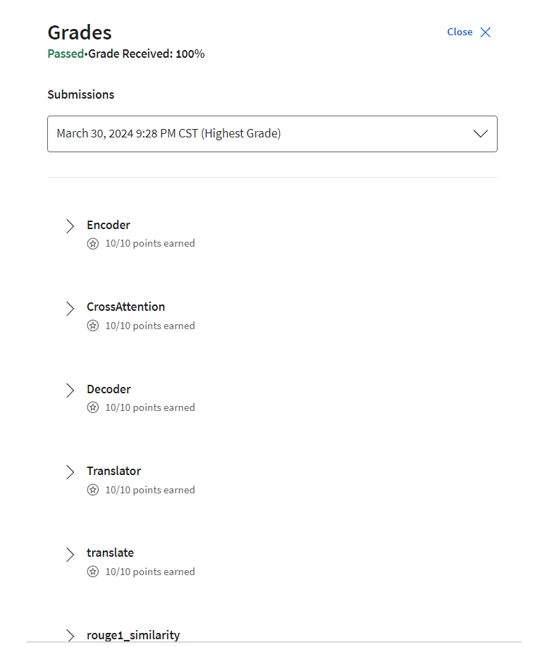
后记
2024年3月30日21点29分完成Week1的Lab,花费1天的时间。这第四门课开始了Attention知识的学习,下周就要讲Transformer,期待一下。
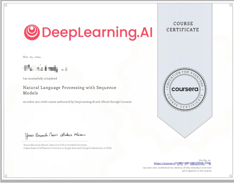


![[数据结构]排序](https://img-blog.csdnimg.cn/direct/07c8817f785643c88d3de4bf6878ef44.png)