Natural Language Processing with Sequence Models
Course Certificate
本文是https://www.coursera.org/learn/sequence-models-in-nlp 这门课程的学习笔记,如有侵权,请联系删除。
文章目录
- Natural Language Processing with Sequence Models
- Week 01: Recurrent Neural Networks for Language Modeling
- Introduction to Neural Networks and TensorFlow
- Lab: Introduction to TensorFlow
- Practice Programming Assignment: Sentiment with Deep Neural Networks
- N-grams vs. Sequence Models
- Practice Quiz: RNNs for Language Modelling
- Programming Assignment: Deep N-grams
-
- Overview
- 1 - Data Preprocessing Overview
-
- 1.1 - Loading in the Data
- 1.2 - Create the vocabulary
- 1.3 - Convert a Line to Tensor
- Exercise 1 - line_to_tensor
- 1.4 - Prepare your data for training and testing
- 1.5 - TensorFlow dataset
- 1.6 - Create the input and the output for your model
- Exercise 2 - create_batch_dataset
- 1.7 - Create the training dataset
- 2 - Defining the GRU Language Model (GRULM)
- 3 - Training
- 4 - Evaluation
- 5 - Generating Language with your Own Model
- Grades
- 后记
Week 01: Recurrent Neural Networks for Language Modeling
Learn about the limitations of traditional language models and see how RNNs and GRUs use sequential data for text prediction. Then build your own next-word generator using a simple RNN on Shakespeare text data!
Learning Objectives
- Supervised machine learning
- Binary classification
- Neural networks
- N-grams
- Gated recurrent units
- Recurrent neural networks
Introduction to Neural Networks and TensorFlow
Neural Networks for Sentiment Analysis
Previously in the course you did sentiment analysis with logistic regression and naive Bayes. Those models were in a sense more naive, and are not able to catch the sentiment off a tweet like: "I am not happy " or “If only it was a good day”. When using a neural network to predict the sentiment of a sentence, you can use the following. Note that the image below has three outputs, in this case you might want to predict, “positive”, "neutral ", or “negative”.
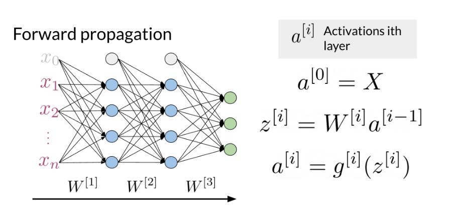
Note that the network above has three layers. To go from one layer to another you can use a W matrix to propagate to the next layer. Hence, we call this concept of going from the input until the final layer, forward propagation. To represent a tweet, you can use the following:
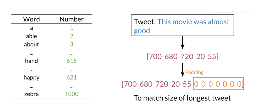
Note, that we add zeros for padding to match the size of the longest tweet.
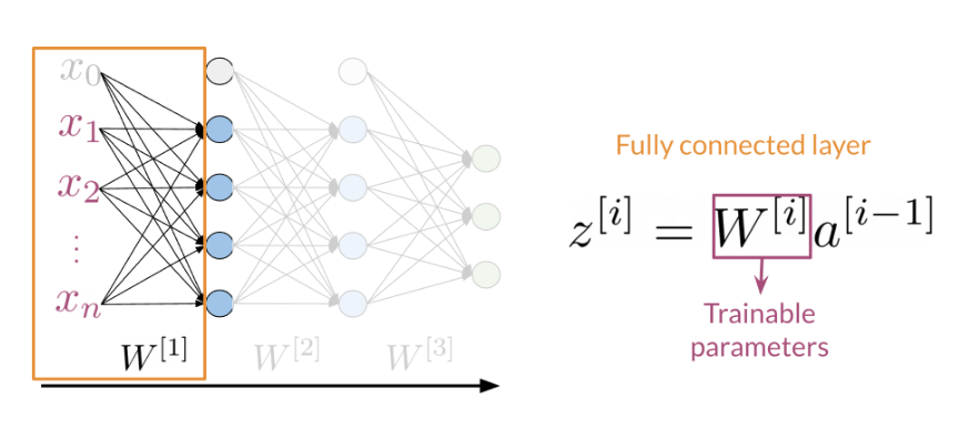
A neural network in the setup you can see above can only process one such tweet at a time. In order to make training more efficient (faster) you want to process many tweets in parallel. You achieve this by putting many tweets together into a matrix and then passing this matrix (rather than individual tweets) through the neural network. Then the neural network can perform its computations on all tweets at the same time.
Dense Layers and ReLU
The Dense layer is the computation of the inner product between a set of trainable weights (weight matrix) and an input vector. The visualization of the dense layer can be seen in the image below.
The orange box in the image above shows the dense layer. An activation layer is the set of blue nodes shown with the orange box in the image below. Concretely one of the most commonly used activation layers is the rectified linear unit (ReLU).
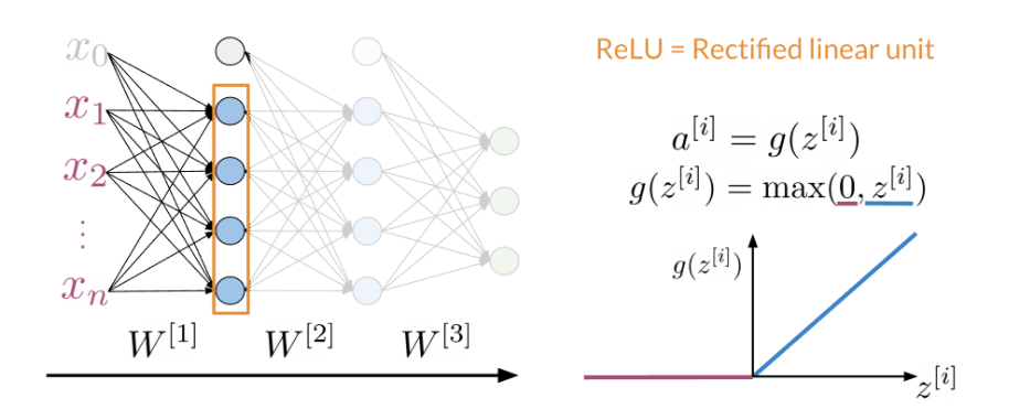
ReLU(x) is defined as max(0,x) for any input x.
Embedding and Mean Layers
Using an embedding layer you can learn word embeddings for each word in your vocabulary as follows:
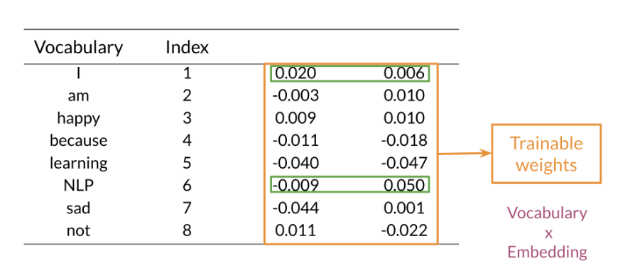
The mean layer allows you to take the average of the embeddings. You can visualize it as follows:
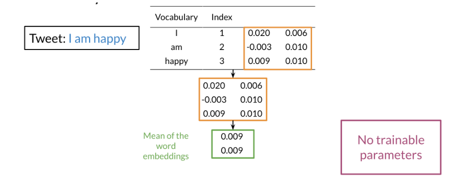
This layer does not have any trainable parameters.
Lab: Introduction to TensorFlow
Lab 1: TensorFlow Tutorial and Some Useful Functions
Welcome to the first lab in this course. Here you will see and try out some basics of TensorFlow and get familiar with some of the useful functions that you will use across the assignments. If you already know TensorFlow well, feel free to skip this notebook.
For the demonstration purposes you will use the IMDB reviews dataset, on which you will perform sentiment classification. The dataset consists of 50,000 movie reviews from the Internet Movie Database (IMDB), but has been shrinked down to 6,000 reviews to save space and ensure faster performance of the notebook.
A part of the code in this notebook is reused from the TensorFlow official tutorial.
1. Import the libraries
# To silence the TensorFlow warnings, you can use the following code before you import the TensorFlow library.
import os
os.environ['TF_CPP_MIN_LOG_LEVEL'] = '3'

import numpy as np
import tensorflow as tf
from tensorflow.keras.preprocessing.text import Tokenizer
from tensorflow.keras import layers
from tensorflow.keras import losses
import re
import string
import matplotlib.pyplot as plt

print("Imports successful!")
Setting the random seed allows you to have control over the (pseudo)random numbers. When you are working with neural networks this is a good idea, so you can get reproducible results (when you run the calculation twice you will always get the same “random” numbers). It is especially important not to mess with the random seed in your assignments, as they are used for checking whether your values are set correctly.
# Select your favourite number for the random seed
seed = 42

# Sets the global random seed for numpy.
np.random.seed(seed)
# Sets the global random seed for TensorFlow.
tf.random.set_seed(seed)

print(f"Random seed set to {seed}")
Output
Random seed set to 42
2. Load the data
First you set the path to the directory where you store your data.
data_dir = './data/aclImdb'
Below, you will use the function tf.keras.utils.text_dataset_from_directory, that generates a tf.data.Dataset from text files in a directory.
TensorFlow allows you for very easy dataset creation, provided that you have data in the following folder substructure.
main_directory/
... class_a/
...... a_text_1.txt
...... a_text_2.txt
... class_b/
...... b_text_1.txt
...... b_text_2.txt
Calling text_dataset_from_directory(...) will return a tf.data.Dataset that yields batches of texts from the subdirectories class_a and class_b, together with labels 0 and 1 (0 corresponding to class_a and 1 corresponding to class_b).
Only .txt files are supported at this time, but there are equivalent functions for different kinds of data, for example image_dataset_from_directory for images.
In your case you have two main directories: ./data/aclImdb/train/ and ./data/aclImdb/test/. Within both of these two directories you have data separated in two classes: neg and pos. So your actual folder structure looks like this:
./data/aclImdb/train/
... neg/
...... text_1.txt
...... text_2.txt
...... ...
... pos/
...... text_1.txt
...... text_2.txt
...... ...
And the same for the test folder, with many .txt files in each subfolder.
You can explore the folders by clicking File and then Open in the menu above, or by clicking on the Jupyter symbol.
In the cell below, you will load the data. Note the different parameters that you can use when loading the data. For example: originally you only have the data split only to training and test sets, but you can very easily split the datasets further, by using just a few parameters.
# Here you have two main directories: one for train and one for test data.
# You load files from each to create training and test datasets.

# Create the training set. Use 80% of the data and keep the remaining 20% for the validation.
raw_training_set = tf.keras.utils.text_dataset_from_directory(
    f'{data_dir}/train',
    labels='inferred',
    label_mode='int',
    batch_size=32,
    validation_split=0.2,
    subset='training',
    seed=seed
)

# Create the validation set. Use 20% of the data that was not used for training.
raw_validation_set = tf.keras.utils.text_dataset_from_directory(
    f'{data_dir}/train',
    labels='inferred',
    label_mode='int',
    batch_size=32,
    validation_split=0.2,
    subset='validation',
    seed=seed
)

# Create the test set.
raw_test_set = tf.keras.utils.text_dataset_from_directory(
    f'{data_dir}/test',
    labels='inferred',
    label_mode='int',
    batch_size=32,
)
Output
Found 5000 files belonging to 2 classes.
Using 4000 files for training.
Found 5000 files belonging to 2 classes.
Using 1000 files for validation.
Found 5000 files belonging to 2 classes.
Check that the labels 0 and 1 correctly correspond to the negative and positive examples respectively.
print(f"Label 0 corresponds to {raw_training_set.class_names[0]}")
print(f"Label 1 corresponds to {raw_training_set.class_names[1]}")
Output
Label 0 corresponds to neg
Label 1 corresponds to pos
If you want to look at a small subset of your dataset, you can use .take() method, by passing it the count parameter. The method returns a new dataset of the size at most count, where count is the number of batches. You can read more about tf.data.Dataset and the take method here.
# Take one batch from the dataset and print out the first three datapoints in the batch
for text_batch, label_batch in raw_training_set.take(1):
    for i in range(3):
        print(f"Review:\n {text_batch.numpy()[i]}")
        print(f"Label: {label_batch.numpy()[i]}\n")
Output
Review:
 b'This is a reunion, a team, and a great episode of Justice. From hesitation to resolution, Clark has made a important leap from a troubled teenager who was afraid of a controlled destiny, to a Superman who, like Green Arrow, sets aside his emotions to his few loved ones, ready to save the whole planet. This is not just a thrilling story about teamwork, loyalty, and friendship; this is also about deciding what\'s more important in life, a lesson for Clark. I do not want the series to end, but I hope the ensuing episodes will strictly stick to what Justice shows without any "rewind" pushes and put a good end here of Smallville---and a wonderful beginning of Superman.<br /><br />In this episode, however, we should have seen more contrast between Lex and the Team. Nine stars should give it enough credit.'
Label: 1

Review:
 b'"Hey Babu Riba" is a film about a young woman, Mariana (nicknamed "Esther" after a famous American movie star), and four young men, Glenn, Sacha, Kicha, and Pop, all perhaps 15-17 years old in 1953 Belgrade, Yugoslavia. The five are committed friends and crazy about jazz, blue jeans, or anything American it seems.<br /><br />The very close relationship of the teenagers is poignant, and ultimately a sacrifice is willingly made to try to help one of the group who has fallen on unexpected difficulties. In the wake of changing communist politics, they go their separate ways and reunite in 1985 (the year before the film was made).<br /><br />I enjoyed the film with some reservations. The subtitles for one thing were difficult. Especially in the beginning, there were a number of dialogues which had no subtitles at all. Perhaps the conversational pace required it, but I couldn\'t always both read the text and absorb the scene, which caused me to not always understand which character was involved. I watched the movie (a video from our public library) with a friend, and neither of us really understood part of the story about acquiring streptomycin for a sick relative.<br /><br />This Yugoslavian coming of age film effectively conveyed the teenagers\' sense of invulnerability, idealism, and strong and loyal bonds to each other. There is a main flashforward, and it was intriguing, keeping me guessing until the end as to who these characters were vis-a-vis the 1953 cast, and what had actually happened.<br /><br />I would rate it 7 out of 10, and would like to see other films by the director, Jovan Acin (1941-1991).'
Label: 1

Review:
 b"No message. No symbolism. No dark undercurrents.Just a wonderful melange of music, nostalgia and good fun put to-gether by people who obviously had a great time doing it. It's a refreshing antidote to some of the pretentious garbage being ground out by the studios. Of course ANYTHING with the incomparable Judi Dench is worth watching. And Cleo Laine's brilliant jazz singing is a bonus. This lady is in the same league as the late Ella. This goes on my movie shelf to be pulled out again anytime I feel the need for a warm experience and a hearty good natured chuckle. Just a wonderful film!"
Label: 1
3. Prepare the Data
Now that you have seen how the dataset looks like, you need to prepare it in the format that a neural network understands. For this, you will use the tf.keras.layers.TextVectorization layer.
This layer converts text to vectors that can then be fed to a neural network. A very useful feature is that you can pass it another function that performs custom standardization of text. This includes lowercasing the text, removing punctuation and/or HTML elements, web links or certain tags. This is very important, as every dataset requires different standardization, depending on its contents. After the standardization, the layer tokenizes the text (splits into words) and vectorizes it (converts from words to numbers) so that it can be fed to the neural network. The output_sequence_length is set to 250, which means that the layer will pad shorter sequences or truncate longer sequences, so they will al have the same length. This is done so that all the inout vectors are the same length and can be nicely put together into matrices.
# Set the maximum number of words
max_features = 10000

# Define the custom standardization function
def custom_standardization(input_data):
    # Convert all text to lowercase
    lowercase = tf.strings.lower(input_data)
    # Remove HTML tags
    stripped_html = tf.strings.regex_replace(lowercase, '<br />', ' ')
    # Remove punctuation
    replaced = tf.strings.regex_replace(
        stripped_html,
        '[%s]' % re.escape(string.punctuation),
        ''
    )
    return replaced

# Create a layer that you can use to convert text to vectors
vectorize_layer = layers.TextVectorization(
    standardize=custom_standardization,
    max_tokens=max_features,
    output_mode='int',
    output_sequence_length=250)
Next, you call adapt to fit the state of the preprocessing layer to the dataset. This will cause the model to build a vocabulary (an index of strings to integers). If you want to access the vocabulary, you can call the .get_vocabulary() on the layer.
# Build the vocabulary
train_text = raw_training_set.map(lambda x, y: x)
vectorize_layer.adapt(train_text)

# Print out the vocabulary size
print(f"Vocabulary size: {len(vectorize_layer.get_vocabulary())}")
raw_training_set.map(lambda x, y: x)解释:
这行代码使用了 TensorFlow 的 map 函数,它将函数应用于数据集中的每个元素。在这里,raw_training_set 是一个数据集,每个元素都是一个 (x, y) 元组,其中 x 是文本数据,y 是对应的标签。Lambda 函数 lambda x, y: x 用于提取每个元组中的文本数据 x,并将其作为输出。因此,train_text 包含了所有训练集中的文本数据。
Output
Vocabulary size: 10000
Now you can define the final function that you will use to vectorize the text and see what it looks like.
Note that you need to add the .expand_dims(). This adds another dimension to your data and is very commonly used when processing data to add an additional dimension to accomodate for the batches.
# Define the final function that you will use to vectorize the text.
def vectorize_text(text, label):
    text = tf.expand_dims(text, -1)
    return vectorize_layer(text), label

# Get one batch and select the first datapoint
text_batch, label_batch = next(iter(raw_training_set))
first_review, first_label = text_batch[0], label_batch[0]

# Show the raw data
print(f"Review:\n{first_review}")
print(f"\nLabel: {raw_training_set.class_names[first_label]}")
# Show the vectorized data
print(f"\nVectorized review\n{vectorize_text(first_review, first_label)}")
Output
Review:
b"Okay, so the plot is on shaky ground. Yeah, all right, so there are some randomly inserted song and/or dance sequences (for example: Adam's concert and Henri's stage act). And Leslie Caron can't really, um, you know... act.<br /><br />But somehow, 'An American In Paris' manages to come through it all as a polished, first-rate musical--largely on the basis of Gene Kelly's incredible dancing talent and choreography, and the truckloads of charm he seems to be importing into each scene with Caron. (He needs to, because she seems to have a... problem with emoting.) <br /><br />The most accomplished and technically awe-inspiring number in this musical is obviously the 16-minute ballet towards the end of the film. It's stunningly filmed, and Kelly and Caron dance beautifully. But my favourite number would have to be Kelly's character singing 'I Got Rhythm' with a bunch of French school-children, then breaking into an array of American dances. It just goes to prove how you don't need special effects when you've got some real *talent*.<br /><br />Not on the 'classics' level with 'Singin' In The Rain', but pretty high up there nonetheless. Worth the watch!"

Label: pos

Vectorized review
(<tf.Tensor: shape=(1, 250), dtype=int64, numpy=
array([[ 947,   38,    2,  112,    7,   20, 6022, 1754, 1438,   31,  201,
          38,   46,   24,   47, 6565, 8919,  603, 2928,  831,  858,   15,
         476, 3241, 3010,    4,    1,  892,  478,    4, 3553, 5885,  175,
          63, 6992,   21,  118,  478,   18,  813,   33,  329,    8, 1466,
        1029,    6,  227,  143,    9,   31,   14,    3, 6590, 9055,    1,
          20,    2, 3025,    5, 1996,    1, 1085,  914,  597,    4, 2733,
           4,    2,    1,    5, 1411,   27,  190,    6,   26,    1,   77,
         244,  130,   16, 5885,   27,  731,    6,   80,   53,  190,    6,
          25,    3,  425,   16,    1,    2,   85, 3622,    4, 2603,    1,
         593,    8,   10,  663,    7,  506,    2,    1, 4342, 1089,    2,
         121,    5,    2,   19,   29, 5994,  886,    4, 1561,    4, 5885,
         831, 1415,   18,   55, 1496,  593,   62,   25,    6,   26,    1,
         105,  965,   11,  186, 4687,   16,    3,  862,    5, 1001,    1,
          96, 2442,   77,   33, 7537,    5,  329, 4825,    9,   41,  264,
           6, 2131,   86,   21,   87,  333,  290,  317,   51,  699,  186,
          47,  144,  597,   23,   20,    2, 2008,  557,   16, 7714,    8,
           2, 2477,   18,  179,  307,   57,   46, 2878,  268,    2,  106,
           0,    0,    0,    0,    0,    0,    0,    0,    0,    0,    0,
           0,    0,    0,    0,    0,    0,    0,    0,    0,    0,    0,
           0,    0,    0,    0,    0,    0,    0,    0,    0,    0,    0,
           0,    0,    0,    0,    0,    0,    0,    0,    0,    0,    0,
           0,    0,    0,    0,    0,    0,    0,    0,    0,    0,    0,
           0,    0,    0,    0,    0,    0,    0,    0]])>, <tf.Tensor: shape=(), dtype=int32, numpy=1>)
Now you can apply the vectorization function to vectorize all three datasets.
train_ds = raw_training_set.map(vectorize_text)
val_ds = raw_validation_set.map(vectorize_text)
test_ds = raw_test_set.map(vectorize_text)
在 TensorFlow 中,map 方法用于对数据集中的每个样本应用一个函数。
Configure the Dataset
There are two important methods that you should use when loading data to make sure that I/O does not become blocking.
.cache() keeps data in memory after it’s loaded off disk. This will ensure the dataset does not become a bottleneck while training your model. If your dataset is too large to fit into memory, you can also use this method to create a performant on-disk cache, which is more efficient to read than many small files.
.prefetch() overlaps data preprocessing and model execution while training.
You can learn more about both methods, as well as how to cache data to disk in the data performance guide.
For very interested, you can read more about tf.data and AUTOTUNE in this paper, but be aware that this is already very advanced information about how TensorFlow works.
AUTOTUNE = tf.data.AUTOTUNE

train_ds = train_ds.cache().prefetch(buffer_size=AUTOTUNE)
test_ds = test_ds.cache().prefetch(buffer_size=AUTOTUNE)
在这段代码中,AUTOTUNE 是一个特殊的值,用于告诉 TensorFlow 在运行时根据可用的计算资源自动选择合适的参数值。tf.data.AUTOTUNE 的值在不同的硬件和工作负载下可能会有所不同,它会根据系统资源(如 CPU 和内存)的状况来自动调整参数。
在这里,cache() 方法将数据集缓存起来,以提高数据加载的效率。缓存数据集可以确保数据在被重复使用时不会重新加载,从而节省了加载时间。
prefetch() 方法用于在训练过程中异步加载数据,以减少训练时的等待时间。buffer_size 参数指定了要预取的样本数。通过调用 prefetch(buffer_size=AUTOTUNE),我们告诉 TensorFlow 在运行时自动选择合适的预取数量,以优化数据加载的性能。
4. Create a Sequential Model
A Sequential model is appropriate for a simple stack of layers where each layer has exactly one input tensor and one output tensor (layers follow each other in a sequence and there are no additional connections).
Here you will use a Sequential model using only three layers:
- An Embedding layer. This layer takes the integer-encoded reviews and looks up an embedding vector for each word-index. These vectors are learned as the model trains. The vectors add a dimension to the output array. The resulting dimensions are: (batch, sequence, embedding).
- A GlobalAveragePooling1D layer returns a fixed-length output vector for each example by averaging over the sequence dimension. This allows the model to handle input of variable length, in the simplest way possible.
- A Dense layer with a single output node.
embedding_dim = 16

# Create the model by calling tf.keras.Sequential, where the layers are given in a list.
model_sequential = tf.keras.Sequential([
    layers.Embedding(max_features, embedding_dim),
    layers.GlobalAveragePooling1D(),
    layers.Dense(1, activation='sigmoid')
])

# Print out the summary of the model
model_sequential.summary()
这段代码使用了 tf.keras.Sequential 来创建一个序列模型,其中包含了几个层:
layers.Embedding(max_features, embedding_dim):这是一个嵌入层,用于将输入的整数序列(每个整数代表一个单词的索引)转换为密集的向量表示。max_features表示词汇表的大小,embedding_dim表示嵌入向量的维度。layers.GlobalAveragePooling1D():这是一个全局平均池化层,用于在时间维度上对输入的一维特征序列进行平均池化,得到一个全局的特征表示。layers.Dense(1, activation='sigmoid'):这是一个全连接层,包含一个神经元,使用 Sigmoid 激活函数。这个层用于将全局池化得到的特征表示映射到一个输出值,通常用于二分类任务。
这个序列模型按照给定的顺序依次堆叠这些层,构建了一个端到端的深度学习模型,用于处理文本数据并执行二分类任务。
Output
Model: "sequential"
_________________________________________________________________
 Layer (type)                Output Shape              Param #
=================================================================
 embedding (Embedding)       (None, None, 16)          160000

 global_average_pooling1d (  (None, 16)                0
 GlobalAveragePooling1D)

 dense (Dense)               (None, 1)                 17

=================================================================
Total params: 160017 (625.07 KB)
Trainable params: 160017 (625.07 KB)
Non-trainable params: 0 (0.00 Byte)
_________________________________________________________________
Compile the model. Choose the loss function, the optimizer and any additional metrics you want to calculate. Since this is a binary classification problem you can use the losses.BinaryCrossentropy loss function.
model_sequential.compile(loss=losses.BinaryCrossentropy(),
              optimizer='adam',
              metrics=['accuracy'])
5. Create a Model Using Functional API
You can use the functional API when you want to create more complex models, but it works just as well for the simple models like the one above. The functional API can handle models with non-linear topology, shared layers, and even multiple inputs or outputs.
The biggest difference at the first glance is that you need to explicitly state the input. Then you use the layers as functions and pass previous layers as parameters into the functions. In the end you build a model, where you pass it the input and the output of the neural network. All of the information from between them (hidden layers) is already hidden in the output layer (remember how each layer takes the previous layer in as a parameter).
# Define the inputs
inputs = tf.keras.Input(shape=(None,))

# Define the first layer
embedding = layers.Embedding(max_features, embedding_dim)
# Call the first layer with inputs as the parameter
x = embedding(inputs)

# Define the second layer
pooling = layers.GlobalAveragePooling1D()
# Call the first layer with the output of the previous layer as the parameter
x = pooling(x)

# Define and call in the same line. (Same thing used two lines of code above
# for other layers. You can use any option you prefer.)
outputs = layers.Dense(1, activation='sigmoid')(x)
#The two-line alternative to the one layer would be:
# dense = layers.Dense(1, activation='sigmoid')
# x = dense(x)


# Create the model
model_functional = tf.keras.Model(inputs=inputs, outputs=outputs)

# Print out the summary of the model
model_functional.summary()
Output
Model: "model"
_________________________________________________________________
 Layer (type)                Output Shape              Param #
=================================================================
 input_1 (InputLayer)        [(None, None)]            0

 embedding_1 (Embedding)     (None, None, 16)          160000

 global_average_pooling1d_1  (None, 16)                0
  (GlobalAveragePooling1D)

 dense_1 (Dense)             (None, 1)                 17

=================================================================
Total params: 160017 (625.07 KB)
Trainable params: 160017 (625.07 KB)
Non-trainable params: 0 (0.00 Byte)
_________________________________________________________________
这个输出的形状描述显示了每个层的输出形状,但不包括批量大小(Batch Size)。在这个例子中,(None, None, 16) 表示第一个维度是批量大小(Batch Size),第二个维度是序列长度(Sequence Length),第三个维度是特征维度(Feature Dimension)。
具体来说:
(None, None)表示输入层(Input Layer)接受的是二维张量,第一个维度为批量大小,第二个维度为序列长度。None表示这两个维度的长度可以是任意值,这取决于输入数据的实际形状。(None, None, 16)表示嵌入层(Embedding Layer)的输出是一个三维张量,第一个维度为批量大小,第二个维度为序列长度,第三个维度为特征维度。在这个例子中,特征维度为16。(None, 16)表示全局平均池化层(Global Average Pooling 1D Layer)的输出是一个二维张量,第一个维度为批量大小,第二个维度为特征维度。在这个例子中,特征维度为16。(None, 1)表示密集连接层(Dense Layer)的输出是一个二维张量,第一个维度为批量大小,第二个维度为神经元数量。在这个例子中,有一个神经元,因此输出的维度为(None, 1)。
因此,这里给出的是每个层的输出形状,而不是输出维度。
Compile the model: choose the loss, optimizer and any additional metrics you want to calculate. This is the same as for the sequential model.
model_functional.compile(loss=losses.BinaryCrossentropy(),
              optimizer='adam',
              metrics=['accuracy'])
6. Train the Model
Above, you have defined two different models: one with a functional api and one sequential model. From now on, you will use only one of them. feel free to change which model you want to use in the next cell. The results should be the same, as the architectures of both models are the same.
# Select which model you want to use and train. the results should be the same
model = model_functional # model = model_sequential
Now you will train the model. You will pass it the training and validation dataset, so it can compute the accuracy metric on both during training.
epochs = 25
history = model.fit(
    train_ds,
    validation_data=val_ds,
    epochs=epochs,
    verbose=2
)
Output
Epoch 1/25
125/125 - 2s - loss: 0.6903 - accuracy: 0.5648 - val_loss: 0.6864 - val_accuracy: 0.6810 - 2s/epoch - 15ms/step
Epoch 2/25
125/125 - 1s - loss: 0.6788 - accuracy: 0.7032 - val_loss: 0.6723 - val_accuracy: 0.7200 - 765ms/epoch - 6ms/step
Epoch 3/25
125/125 - 1s - loss: 0.6582 - accuracy: 0.7460 - val_loss: 0.6501 - val_accuracy: 0.7420 - 769ms/epoch - 6ms/step
Epoch 4/25
125/125 - 1s - loss: 0.6295 - accuracy: 0.7753 - val_loss: 0.6224 - val_accuracy: 0.7680 - 658ms/epoch - 5ms/step
Epoch 5/25
125/125 - 1s - loss: 0.5958 - accuracy: 0.7920 - val_loss: 0.5931 - val_accuracy: 0.7860 - 644ms/epoch - 5ms/step
Epoch 6/25
125/125 - 1s - loss: 0.5604 - accuracy: 0.8102 - val_loss: 0.5645 - val_accuracy: 0.7980 - 649ms/epoch - 5ms/step
Epoch 7/25
125/125 - 1s - loss: 0.5251 - accuracy: 0.8335 - val_loss: 0.5377 - val_accuracy: 0.8020 - 659ms/epoch - 5ms/step
Epoch 8/25
125/125 - 1s - loss: 0.4912 - accuracy: 0.8530 - val_loss: 0.5129 - val_accuracy: 0.8070 - 640ms/epoch - 5ms/step
Epoch 9/25
125/125 - 1s - loss: 0.4592 - accuracy: 0.8712 - val_loss: 0.4905 - val_accuracy: 0.8190 - 784ms/epoch - 6ms/step
Epoch 10/25
125/125 - 1s - loss: 0.4294 - accuracy: 0.8832 - val_loss: 0.4703 - val_accuracy: 0.8260 - 695ms/epoch - 6ms/step
Epoch 11/25
125/125 - 1s - loss: 0.4020 - accuracy: 0.8932 - val_loss: 0.4524 - val_accuracy: 0.8330 - 633ms/epoch - 5ms/step
Epoch 12/25
125/125 - 1s - loss: 0.3769 - accuracy: 0.9025 - val_loss: 0.4366 - val_accuracy: 0.8430 - 659ms/epoch - 5ms/step
Epoch 13/25
125/125 - 1s - loss: 0.3540 - accuracy: 0.9065 - val_loss: 0.4227 - val_accuracy: 0.8470 - 609ms/epoch - 5ms/step
Epoch 14/25
125/125 - 1s - loss: 0.3331 - accuracy: 0.9143 - val_loss: 0.4105 - val_accuracy: 0.8490 - 620ms/epoch - 5ms/step
Epoch 15/25
125/125 - 1s - loss: 0.3140 - accuracy: 0.9233 - val_loss: 0.3998 - val_accuracy: 0.8580 - 624ms/epoch - 5ms/step
Epoch 16/25
125/125 - 1s - loss: 0.2965 - accuracy: 0.9293 - val_loss: 0.3903 - val_accuracy: 0.8560 - 655ms/epoch - 5ms/step
Epoch 17/25
125/125 - 1s - loss: 0.2804 - accuracy: 0.9327 - val_loss: 0.3820 - val_accuracy: 0.8560 - 673ms/epoch - 5ms/step
Epoch 18/25
125/125 - 1s - loss: 0.2654 - accuracy: 0.9377 - val_loss: 0.3747 - val_accuracy: 0.8560 - 718ms/epoch - 6ms/step
Epoch 19/25
125/125 - 1s - loss: 0.2515 - accuracy: 0.9427 - val_loss: 0.3683 - val_accuracy: 0.8580 - 659ms/epoch - 5ms/step
Epoch 20/25
125/125 - 1s - loss: 0.2385 - accuracy: 0.9467 - val_loss: 0.3626 - val_accuracy: 0.8630 - 632ms/epoch - 5ms/step
Epoch 21/25
125/125 - 1s - loss: 0.2263 - accuracy: 0.9513 - val_loss: 0.3576 - val_accuracy: 0.8630 - 644ms/epoch - 5ms/step
Epoch 22/25
125/125 - 1s - loss: 0.2149 - accuracy: 0.9540 - val_loss: 0.3531 - val_accuracy: 0.8620 - 649ms/epoch - 5ms/step
Epoch 23/25
125/125 - 1s - loss: 0.2041 - accuracy: 0.9582 - val_loss: 0.3492 - val_accuracy: 0.8630 - 657ms/epoch - 5ms/step
Epoch 24/25
125/125 - 1s - loss: 0.1939 - accuracy: 0.9622 - val_loss: 0.3458 - val_accuracy: 0.8630 - 682ms/epoch - 5ms/step
Epoch 25/25
125/125 - 1s - loss: 0.1842 - accuracy: 0.9643 - val_loss: 0.3428 - val_accuracy: 0.8620 - 832ms/epoch - 7ms/step
Now you can use model.evaluate() to evaluate the model on the test dataset.
loss, accuracy = model.evaluate(test_ds)

print(f"Loss: {loss}")
print(f"Accuracy: {accuracy}")
Output
157/157 [==============================] - 1s 8ms/step - loss: 0.3642 - accuracy: 0.8452
Loss: 0.36415866017341614
Accuracy: 0.8452000021934509
When you trained the model, you saved the history in the history variable. Here you can access a dictionary that contains everything that happened during the training. In your case it saves the losses and the accuracy on both training and validation sets. You can plot it to gain some insights into how the training is progressing.
def plot_metrics(history, metric):
    plt.plot(history.history[metric])
    plt.plot(history.history[f'val_{metric}'])
    plt.xlabel("Epochs")
    plt.ylabel(metric.title())
    plt.legend([metric, f'val_{metric}'])
    plt.show()

plot_metrics(history, "accuracy")
plot_metrics(history, "loss")
Output
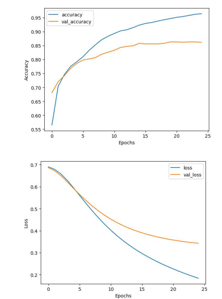
You can see that after 25 epochs, the training accuracy still goes up, but the validation accuracy already plateaus at around 86%. On the other hand both training and validation losses are still decreasing, which means that while the model does not learn to predict more cases accurately, it still gets more confident in its predictions. Here you used the simplest possible model: you have used embeddings, averaging layer and a dense layer with one output. You can try different architectures to see if the model improves. Perhaps you can add some dropout layers to reduce the chance of overfitting, or you can try a completely different architecture, like using convolutional layers or reccurent layers. You will learn a lot more about recurrent neural networks in the later weeks of this course.
7. Predict on Your Own Data
Finally, you can use the model to predict on any new data you may have. You can use it to predict the sentiment of examples in the test dataset (which the model has not seen in the training process) or use some completely new examples.
Here you will expand your model to be able to predict on raw strings (rather than on vectorized examples). Previously, you applied the TextVectorization layer to the dataset before feeding it to the model. To simplify deploying the model, you can include the TextVectorization layer inside your model and then predict on raw strings. To do so, you can create a new sequential model where you merge the vectorization layer with your trained model using the weights you just trained.
# Make a new sequential model using the vectorization layer and the model you just trained.
export_model = tf.keras.Sequential([
  vectorize_layer,
  model]
)

# Compile the model
export_model.compile(
    loss=losses.BinaryCrossentropy(from_logits=False), optimizer="adam", metrics=['accuracy']
)
Now you can use this model to predict on some of your own examples. You can do it simply by calling model.predict()
examples = ['this movie was very, very good', 'quite ok', 'the movie was not bad', 'bad', 'negative disappointed bad scary', 'this movie was stupid']

results = export_model.predict(examples, verbose=False)

for result, example in zip(results, examples):
    print(f'Result: {result[0]:.3f},   Label: {int(np.round(result[0]))},   Review: {example}')
Output
Result: 0.625,   Label: 1,   Review: this movie was very, very good
Result: 0.542,   Label: 1,   Review: quite ok
Result: 0.426,   Label: 0,   Review: the movie was not bad
Result: 0.472,   Label: 0,   Review: bad
Result: 0.427,   Label: 0,   Review: negative disappointed bad scary
Result: 0.455,   Label: 0,   Review: this movie was stupid
Congratulations on finishing this lab. Do not worry if you did not understand everything, the videos and course material will cover these concepts in more depth. If you have a general understanding of the code in this lab, you are very well suited to start working on this weeks programming assignment. There you will implement some of the things shown in this lab from scratch and then create and fit a similar model like you did in this notebook.
Practice Programming Assignment: Sentiment with Deep Neural Networks
Assignment 1: Sentiment with Deep Neural Networks
Welcome to the first assignment of course 3. This is a practice assignment, which means that the grade you receive won’t count towards your final grade of the course. However you can still submit your solutions and receive a grade along with feedback from the grader. Before getting started take some time to read the following tips:
TIPS FOR SUCCESSFUL GRADING OF YOUR ASSIGNMENT:
All cells are frozen except for the ones where you need to submit your solutions.
You can add new cells to experiment but these will be omitted by the grader, so don’t rely on newly created cells to host your solution code, use the provided places for this.
You can add the comment # grade-up-to-here in any graded cell to signal the grader that it must only evaluate up to that point. This is helpful if you want to check if you are on the right track even if you are not done with the whole assignment. Be sure to remember to delete the comment afterwards!
To submit your notebook, save it and then click on the blue submit button at the beginning of the page.
In this assignment, you will explore sentiment analysis using deep neural networks.
In course 1, you implemented Logistic regression and Naive Bayes for sentiment analysis. Even though the two models performed very well on the dataset of tweets, they fail to catch any meaning beyond the meaning of words. For this you can use neural networks. In this assignment, you will write a program that uses a simple deep neural network to identify sentiment in text. By completing this assignment, you will:
- Understand how you can design a neural network using tensorflow
- Build and train a model
- Use a binary cross-entropy loss function
- Compute the accuracy of your model
- Predict using your own input
As you can tell, this model follows a similar structure to the one you previously implemented in the second course of this specialization.
- Indeed most of the deep nets you will be implementing will have a similar structure. The only thing that changes is the model architecture, the inputs, and the outputs. In this assignment, you will first create the neural network layers from scratch using
numpyto better understand what is going on. After this you will use the librarytensorflowfor building and training the model.
1 - Import the Libraries
Run the next cell to import the Python packages you’ll need for this assignment.
Note the from utils import ... line. This line imports the functions that were specifically written for this assignment. If you want to look at what these functions are, go to File -> Open... and open the utils.py file to have a look.
import os
os.environ['TF_CPP_MIN_LOG_LEVEL'] = '3'

import numpy as np
import tensorflow as tf
import matplotlib.pyplot as plt
from sklearn.decomposition import PCA

from utils import load_tweets, process_tweet

%matplotlib inline

import w1_unittest
process_tweet函数如下:
import string
import re
import nltk
nltk.download('twitter_samples')
nltk.download('stopwords')
nltk.download('averaged_perceptron_tagger')
nltk.download('wordnet')

from nltk.tokenize import TweetTokenizer
from nltk.corpus import stopwords, twitter_samples, wordnet
from nltk.stem import WordNetLemmatizer

stopwords_english = stopwords.words('english')
lemmatizer = WordNetLemmatizer()


def process_tweet(tweet):
    '''
    Input:
        tweet: a string containing a tweet
    Output:
        tweets_clean: a list of words containing the processed tweet

    '''
    # remove stock market tickers like $GE
    tweet = re.sub(r'\$\w*', '', tweet)
    # remove old style retweet text "RT"
    tweet = re.sub(r'^RT[\s]+', '', tweet)
    # remove hyperlinks
    tweet = re.sub(r'https?:\/\/.*[\r\n]*', '', tweet)
    # remove hashtags
    # only removing the hash # sign from the word
    tweet = re.sub(r'#', '', tweet)
    # tokenize tweets
    tokenizer = TweetTokenizer(preserve_case=False, strip_handles=True, reduce_len=True)
    tweet_tokens = nltk.pos_tag(tokenizer.tokenize(tweet))

    tweets_clean = []
    for word in tweet_tokens:
        if (word[0] not in stopwords_english and # remove stopwords
            word[0] not in string.punctuation): # remove punctuation
            stem_word = lemmatizer.lemmatize(word[0], pos_tag_convert(word[1]))
            tweets_clean.append(stem_word)
    return tweets_clean


def pos_tag_convert(nltk_tag: str) -> str:
    '''Converts nltk tags to tags that are understandable by the lemmatizer.

    Args:
        nltk_tag (str): nltk tag

    Returns:
        _ (str): converted tag
    '''
    if nltk_tag.startswith('J'):
        return wordnet.ADJ
    elif nltk_tag.startswith('V'):
        return wordnet.VERB
    elif nltk_tag.startswith('N'):
        return wordnet.NOUN
    elif nltk_tag.startswith('R'):
        return wordnet.ADV
    else:
        return wordnet.NOUN


def load_tweets():
    all_positive_tweets = twitter_samples.strings('positive_tweets.json')
    all_negative_tweets = twitter_samples.strings('negative_tweets.json')
    return all_positive_tweets, all_negative_tweets
2 - Import the Data
2.1 - Load and split the Data
- Import the positive and negative tweets
- Have a look at some examples of the tweets
- Split the data into the training and validation sets
- Create labels for the data
# Load positive and negative tweets
all_positive_tweets, all_negative_tweets = load_tweets()

# View the total number of positive and negative tweets.
print(f"The number of positive tweets: {len(all_positive_tweets)}")
print(f"The number of negative tweets: {len(all_negative_tweets)}")
Output
The number of positive tweets: 5000
The number of negative tweets: 5000
Now you can have a look at some examples of tweets.
# Change the tweet number to any number between 0 and 4999 to see a different pair of tweets.
tweet_number = 4
print('Positive tweet example:')
print(all_positive_tweets[tweet_number])
print('\nNegative tweet example:')
print(all_negative_tweets[tweet_number])
Output
Positive tweet example:
yeaaaah yippppy!!!  my accnt verified rqst has succeed got a blue tick mark on my fb profile :) in 15 days

Negative tweet example:
Dang starting next week I have "work" :(
Here you will process the tweets. This part of the code has been implemented for you. The processing includes:
- tokenizing the sentence (splitting to words)
- removing stock market tickers like $GE
- removing old style retweet text “RT”
- removing hyperlinks
- removing hashtags
- lowercasing
- removing stopwords and punctuation
- stemming
Some of these things are general steps you would do when processing any text, some others are very “tweet-specific”. The details of the process_tweet function are available in utils.py file
# Process all the tweets: tokenize the string, remove tickers, handles, punctuation and stopwords, stem the words
all_positive_tweets_processed = [process_tweet(tweet) for tweet in all_positive_tweets]
all_negative_tweets_processed = [process_tweet(tweet) for tweet in all_negative_tweets]
Now you can have a look at some examples of how the tweets look like after being processed.
# Change the tweet number to any number between 0 and 4999 to see a different pair of tweets.
tweet_number = 4
print('Positive processed tweet example:')
print(all_positive_tweets_processed[tweet_number])
print('\nNegative processed tweet example:')
print(all_negative_tweets_processed[tweet_number])
Output
Positive processed tweet example:
['yeaaah', 'yipppy', 'accnt', 'verify', 'rqst', 'succeed', 'get', 'blue', 'tick', 'mark', 'fb', 'profile', ':)', '15', 'day']

Negative processed tweet example:
['dang', 'start', 'next', 'week', 'work', ':(']
Next, you split the tweets into the training and validation datasets. For this example you can use 80 % of the data for training and 20 % of the data for validation.
# Split positive set into validation and training
val_pos = all_positive_tweets_processed[4000:]
train_pos = all_positive_tweets_processed[:4000]
# Split negative set into validation and training
val_neg = all_negative_tweets_processed[4000:]
train_neg = all_negative_tweets_processed[:4000]

train_x = train_pos + train_neg
val_x  = val_pos + val_neg

# Set the labels for the training and validation set (1 for positive, 0 for negative)
train_y = [[1] for _ in train_pos] + [[0] for _ in train_neg]
val_y  = [[1] for _ in val_pos] + [[0] for _ in val_neg]

print(f"There are {len(train_x)} sentences for training.")
print(f"There are {len(train_y)} labels for training.\n")
print(f"There are {len(val_x)} sentences for validation.")
print(f"There are {len(val_y)} labels for validation.")
Output
There are 8000 sentences for training.
There are 8000 labels for training.

There are 2000 sentences for validation.
There are 2000 labels for validation.
2.2 - Build the Vocabulary
Now build the vocabulary.
- Map each word in each tweet to an integer (an “index”).
- Note that you will build the vocabulary based on the training data.
- To do so, you will assign an index to every word by iterating over your training set.
The vocabulary will also include some special tokens
'': padding'[UNK]': a token representing any word that is not in the vocabulary.
Exercise 1 - build_vocabulary
Build the vocabulary from all of the tweets in the training set.
# GRADED FUNCTION: build_vocabulary
def build_vocabulary(corpus):
    '''Function that builds a vocabulary from the given corpus
    Input:
        - corpus (list): the corpus
    Output:
        - vocab (dict): Dictionary of all the words in the corpus.
                The keys are the words and the values are integers.
    '''

    # The vocabulary includes special tokens like padding token and token for unknown words
    # Keys are words and values are distinct integers (increasing by one from 0)
    vocab = {'': 0, '[UNK]': 1}

    ### START CODE HERE ###

    # For each tweet in the training set
    for tweet in corpus:
        # For each word in the tweet
        for word in tweet:
            # If the word is not in vocabulary yet, add it to vocabulary
            if word not in vocab:
                vocab[word] = len(vocab)

    ### END CODE HERE ###

    return vocab


vocab = build_vocabulary(train_x)
num_words = len(vocab)

print(f"Vocabulary contains {num_words} words\n")
print(vocab)
The dictionary Vocab will look like this:
{'': 0,
 '[UNK]': 1,
 'followfriday': 2,
 'top': 3,
 'engage': 4,
 ...
- Each unique word has a unique integer associated with it.
- The total number of words in Vocab: 9535
# Test the build_vocabulary function
w1_unittest.test_build_vocabulary(build_vocabulary)
Output
All tests passed
2.3 - Convert a Tweet to a Tensor
Next, you will write a function that will convert each tweet to a tensor (a list of integer IDs representing the processed tweet).
- You already transformed each tweet to a list of tokens with the
process_tweetfunction in order to make a vocabulary. - Now you will transform the tokens to integers and pad the tensors so they all have equal length.
- Note, the returned data type will be a regular Python
list()- You won’t use TensorFlow in this function
- You also won’t use a numpy array
- For words in the tweet that are not in the vocabulary, set them to the unique ID for the token
[UNK].
Example
You had the original tweet:
'@happypuppy, is Maria happy?'
The tweet is already converted into a list of tokens (including only relevant words).
['maria', 'happy']
Now you will convert each word into its unique integer.
[1, 55]
- Notice that the word “maria” is not in the vocabulary, so it is assigned the unique integer associated with the
[UNK]token, because it is considered “unknown.”
After that, you will pad the tweet with zeros so that all the tweets have the same length.
[1, 56, 0, 0, ... , 0]
First, let’s have a look at the length of the processed tweets. You have to look at all tweets in the training and validation set and find the longest one to pad all of them to the maximum length.
# Tweet lengths
plt.hist([len(t) for t in train_x + val_x]);
Output
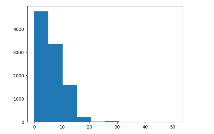
Now find the length of the longest tweet. Remember to look at the training and the validation set.
Exercise 2 - max_len
Calculate the length of the longest tweet.
# GRADED FUNCTION: max_length
def max_length(training_x, validation_x):
    """Computes the length of the longest tweet in the training and validation sets.

    Args:
        training_x (list): The tweets in the training set.
        validation_x (list): The tweets in the validation set.

    Returns:
        int: Length of the longest tweet.
    """
    ### START CODE HERE ###

    max_len = 0

    for tweet in training_x:
        max_len = max(max_len, len(tweet))

    for tweet in validation_x:
        max_len = max(max_len, len(tweet))

    ### END CODE HERE ###
    return max_len

max_len = max_length(train_x, val_x)
print(f'The length of the longest tweet is {max_len} tokens.')
Output
The length of the longest tweet is 51 tokens.
Expected output:
The length of the longest tweet is 51 tokens.
# Test your max_len function
w1_unittest.test_max_length(max_length)
Output
All tests passed
Exercise 3 - padded_sequence
Implement padded_sequence function to transform sequences of words into padded sequences of numbers. A couple of things to notice:
- The term
tensoris used to refer to the encoded tweet but the function should return a regular python list, not atf.tensor - There is no need to truncate the tweet if it exceeds
max_lenas you already know the maximum length of the tweets beforehand
# GRADED FUNCTION: padded_sequence
def padded_sequence(tweet, vocab_dict, max_len, unk_token='[UNK]'):
    """transform sequences of words into padded sequences of numbers

    Args:
        tweet (list): A single tweet encoded as a list of strings.
        vocab_dict (dict): Vocabulary.
        max_len (int): Length of the longest tweet.
        unk_token (str, optional): Unknown token. Defaults to '[UNK]'.

    Returns:
        list: Padded tweet encoded as a list of int.
    """
    ### START CODE HERE ###

    # Find the ID of the UNK token, to use it when you encounter a new word
    unk_ID = vocab_dict[unk_token]

    # First convert the words to integers by looking up the vocab_dict
    # padded_tensor = []
    #for token in tweet:
    #   padded_tensor.append(vocab_dict[token])
    padded_tensor = [vocab_dict.get(word, unk_ID) for word in tweet]
    # Then pad the tensor with zeroes up to the length max_len
    padded_tensor += [0] * (max_len - len(padded_tensor))

    ### END CODE HERE ###

    return padded_tensor
# Test your padded_sequence function
w1_unittest.test_padded_sequence(padded_sequence)
Output
All tests passed
Pad the train and validation dataset
train_x_padded = [padded_sequence(x, vocab, max_len) for x in train_x]
val_x_padded = [padded_sequence(x, vocab, max_len) for x in val_x]
3 - Define the structure of the neural network layers
In this part, you will write your own functions and layers for the neural network to test your understanding of the implementation. It will be similar to the one used in Keras and PyTorch. Writing your own small framework will help you understand how they all work and use them effectively in the future.
You will implement the ReLU and sigmoid functions, which you will use as activation functions for the neural network, as well as a fully connected (dense) layer.
3.1 - ReLU
You will now implement the ReLU activation in a function below. The ReLU function looks as follows:
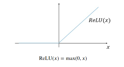
R e L U ( x ) = m a x ( 0 , x ) \mathrm{ReLU}(x) = \mathrm{max}(0,x) ReLU(x)=max(0,x)
Exercise 4 - relu
Instructions: Implement the ReLU activation function below. Your function should take in a matrix or vector and it should transform all the negative numbers into 0 while keeping all the positive numbers intact.
Notice you can get the maximum of two numbers by using np.maximum.
# GRADED FUNCTION: relu
def relu(x):
    '''Relu activation function implementation
    Input:
        - x (numpy array)
    Output:
        - activation (numpy array): input with negative values set to zero
    '''
    ### START CODE HERE ###

    activation = np.maximum(0, x)

    ### END CODE HERE ###

    return activation
# Check the output of your function
x = np.array([[-2.0, -1.0, 0.0], [0.0, 1.0, 2.0]], dtype=float)
print("Test data is:")
print(x)
print("\nOutput of relu is:")
print(relu(x))
Output
Test data is:
[[-2. -1.  0.]
 [ 0.  1.  2.]]

Output of relu is:
[[0. 0. 0.]
 [0. 1. 2.]]
Expected Output:
Test data is:
[[-2. -1.  0.]
 [ 0.  1.  2.]]

Output of relu is:
[[0. 0. 0.]
 [0. 1. 2.]]
# Test your relu function
w1_unittest.test_relu(relu)
Output
All tests passed
3.2 - Sigmoid
You will now implement the sigmoid activation in a function below. The sigmoid function looks as follows:
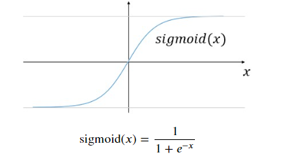
s i g m o i d ( x ) = 1 1 + e − x \mathrm{sigmoid}(x) = \frac{1}{1 + e^{-x}} sigmoid(x)=1+e−x1
Exercise 5 - sigmoid
Instructions: Implement the sigmoid activation function below. Your function should take in a matrix or vector and it should transform all the numbers according to the formula above.
# GRADED FUNCTION: sigmoid
def sigmoid(x):
    '''Sigmoid activation function implementation
    Input:
        - x (numpy array)
    Output:
        - activation (numpy array)
    '''
    ### START CODE HERE ###

    activation = 1 / (1 + np.exp(-x))

    ### END CODE HERE ###

    return activation
# Check the output of your function
x = np.array([[-1000.0, -1.0, 0.0], [0.0, 1.0, 1000.0]], dtype=float)
print("Test data is:")
print(x)
print("\nOutput of sigmoid is:")
print(sigmoid(x))
Output
Test data is:
[[-1000.    -1.     0.]
 [    0.     1.  1000.]]

Output of sigmoid is:
[[0.         0.26894142 0.5       ]
 [0.5        0.73105858 1.        ]]
Expected Output:
Test data is:
[[-1000.    -1.     0.]
 [    0.     1.  1000.]]

Output of sigmoid is:
[[0.         0.26894142 0.5       ]
 [0.5        0.73105858 1.        ]]
# Test your sigmoid function
w1_unittest.test_sigmoid(sigmoid)
Output: All tests passed
3.3 - Dense Class
Implement the weight initialization in the __init__ method.
- Weights are initialized with a random key.
- The shape of the weights (num_rows, num_cols) should equal the number of columns in the input data (this is in the last column) and the number of units respectively.
- The number of rows in the weight matrix should equal the number of columns in the input data
x. Sincexmay have 2 dimensions if it represents a single training example (row, col), or three dimensions (batch_size, row, col), get the last dimension from the tuple that holds the dimensions of x. - The number of columns in the weight matrix is the number of units chosen for that dense layer.
- The number of rows in the weight matrix should equal the number of columns in the input data
- The values generated should have a mean of 0 and standard deviation of
stdev.- To initialize random weights, a random generator is created using
random_generator = np.random.default_rng(seed=random_seed). This part is implemented for you. You will userandom_generator.normal(...)to create your random weights. Check here how the random generator works. - Please don’t change the
random_seed, so that the results are reproducible for testing (and you can be fairly graded).
- To initialize random weights, a random generator is created using
Implement the forward function of the Dense class.
- The forward function multiplies the input to the layer (
x) by the weight matrix (W)
f o r w a r d ( x , W ) = x W \mathrm{forward}(\mathbf{x},\mathbf{W}) = \mathbf{xW} forward(x,W)=xW
- You can use
numpy.dotto perform the matrix multiplication.
Exercise 6 - Dense
Implement the Dense class. You might want to check how normal random numbers can be generated with numpy by checking the docs.
# GRADED CLASS: Dense
class Dense():
    """
    A dense (fully-connected) layer.
    """

    # Please implement '__init__'
    def __init__(self, n_units, input_shape, activation, stdev=0.1, random_seed=42):

        # Set the number of units in this layer
        self.n_units = n_units
        # Set the random key for initializing weights
        self.random_generator = np.random.default_rng(seed=random_seed)
        self.activation = activation

        ### START CODE HERE ###

        # Generate the weight matrix from a normal distribution and standard deviation of 'stdev'
        # Set the size of the matrix w
        w = self.random_generator.normal(scale=stdev, size = (input_shape[-1], n_units))

        ### END CODE HERE ##

        self.weights = w


    def __call__(self, x):
        return self.forward(x)


    # Please implement 'forward()'
    def forward(self, x):

        ### START CODE HERE ###

        # Matrix multiply x and the weight matrix
        dense = np.dot(x, self.weights)
        # Apply the activation function
        dense = self.activation(dense)

        ### END CODE HERE ###
        return dense
# random_key = np.random.get_prng()  # sets random seed
z = np.array([[2.0, 7.0, 25.0]]) # input array

# Testing your Dense layer
dense_layer = Dense(n_units=10, input_shape=z.shape, activation=relu)  #sets  number of units in dense layer

print("Weights are:\n",dense_layer.weights) #Returns randomly generated weights
print("Foward function output is:", dense_layer(z)) # Returns multiplied values of units and weights
Output
Weights are:
 [[ 0.03047171 -0.10399841  0.07504512  0.09405647 -0.19510352 -0.13021795
   0.01278404 -0.03162426 -0.00168012 -0.08530439]
 [ 0.0879398   0.07777919  0.00660307  0.11272412  0.04675093 -0.08592925
   0.03687508 -0.09588826  0.08784503 -0.00499259]
 [-0.01848624 -0.06809295  0.12225413 -0.01545295 -0.04283278 -0.03521336
   0.05323092  0.03654441  0.04127326  0.0430821 ]]
Foward function output is: [[0.21436609 0.         3.25266507 0.59085808 0.         0.
  1.61446659 0.17914382 1.64338651 0.87149558]]
Expected Output:
Weights are:
 [[ 0.03047171 -0.10399841  0.07504512  0.09405647 -0.19510352 -0.13021795
   0.01278404 -0.03162426 -0.00168012 -0.08530439]
 [ 0.0879398   0.07777919  0.00660307  0.11272412  0.04675093 -0.08592925
   0.03687508 -0.09588826  0.08784503 -0.00499259]
 [-0.01848624 -0.06809295  0.12225413 -0.01545295 -0.04283278 -0.03521336
   0.05323092  0.03654441  0.04127326  0.0430821 ]]

Foward function output is: [[0.21436609 0.         3.25266507 0.59085808 0.         0.
  1.61446659 0.17914382 1.64338651 0.87149558]]
# Test your Dense class
w1_unittest.test_Dense(Dense)
Output: All tests passed
3.4 - Model
Now you will implement a classifier using neural networks. Here is the model architecture you will be implementing.
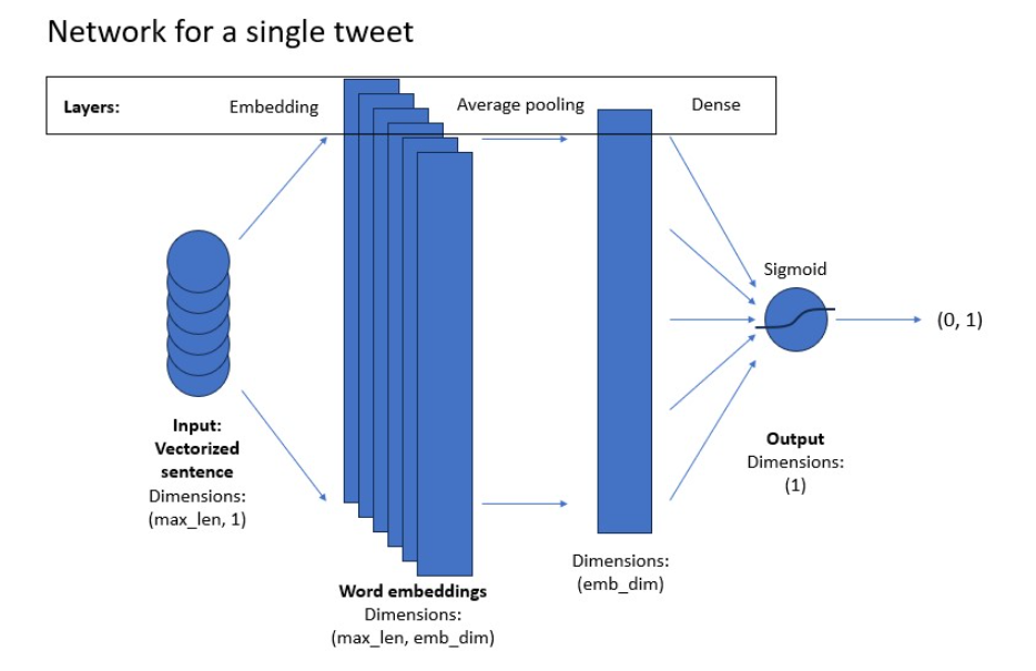
For the model implementation, you will use TensorFlow module, imported as tf. Your model will consist of layers and activation functions that you implemented above, but you will take them directly from the tensorflow library.
You will use the tf.keras.Sequential module, which allows you to stack the layers in a sequence as you want them in the model. You will use the following layers:
- tf.keras.layers.Embedding
- Turns positive integers (word indices) into vectors of fixed size. You can imagine it as creating one-hot vectors out of indices and then running them through a fully-connected (dense) layer.
- tf.keras.layers.GlobalAveragePooling1D
- tf.keras.layers.Dense
- Regular fully connected layer
Please use the help function to view documentation for each layer.
# View documentation on how to implement the layers in tf.
# help(tf.keras.Sequential)
# help(tf.keras.layers.Embedding)
# help(tf.keras.layers.GlobalAveragePooling1D)
# help(tf.keras.layers.Dense)
Exercise 7 - create_model
Implement the create_model function.
First you need to create the model. The tf.keras.Sequential has been implemented for you. Within it you should put the following layers:
tf.keras.layers.Embeddingwith the sizenum_wordstimesembeding_dimand theinput_lengthset to the length of the input sequences (which is the length of the longest tweet).tf.keras.layers.GlobalAveragePooling1Dwith no extra parameters.tf.keras.layers.Densewith the size of one (this is your classification output) and'sigmoid'activation passed to theactivationkeyword parameter.
Make sure to separate the layers with a comma.
Then you need to compile the model. Here you can look at all the parameters you can set when compiling the model: tf.keras.Model. In this notebook, you just need to set the loss to 'binary_crossentropy' (because you are doing binary classification with a sigmoid function at the output), the optimizer to 'adam' and the metrics to 'accuracy' (so that you can track the accuracy on the training and validation sets.
# GRADED FUNCTION: create_model
def create_model(num_words, embedding_dim, max_len):
    """
    Creates a text classifier model

    Args:
        num_words (int): size of the vocabulary for the Embedding layer input
        embedding_dim (int): dimensionality of the Embedding layer output
        max_len (int): length of the input sequences

    Returns:
        model (tf.keras Model): the text classifier model
    """

    tf.random.set_seed(123)

    ### START CODE HERE

    model = tf.keras.Sequential([
        tf.keras.layers.Embedding(num_words, embedding_dim, input_length=max_len),
        tf.keras.layers.GlobalAveragePooling1D(),
        tf.keras.layers.Dense(1, activation="sigmoid")
    ])

    model.compile(loss="binary_crossentropy",
                  optimizer="adam",
                  metrics=['accuracy'])

    ### END CODE HERE

    return model
# Create the model
model = create_model(num_words=num_words, embedding_dim=16, max_len=max_len)

print('The model is created!\n')
Output: The model is created!
# Test your create_model function
w1_unittest.test_model(create_model)
Output: All tests passed
Now you need to prepare the data to put into the model. You already created lists of x and y values and all you need to do now is convert them to NumPy arrays, as this is the format that the model is expecting.
Then you can create a model with the function you defined above and train it. The trained model should give you about 99.6 % accuracy on the validation set.
# Prepare the data
train_x_prepared = np.array(train_x_padded)
val_x_prepared = np.array(val_x_padded)

train_y_prepared = np.array(train_y)
val_y_prepared = np.array(val_y)

print('The data is prepared for training!\n')

# Fit the model
print('Training:')
history = model.fit(train_x_prepared, train_y_prepared, epochs=20, validation_data=(val_x_prepared, val_y_prepared))
Output
The data is prepared for training!

Training:
Epoch 1/20
250/250 [==============================] - 16s 53ms/step - loss: 0.6841 - accuracy: 0.6506 - val_loss: 0.6695 - val_accuracy: 0.9755
Epoch 2/20
250/250 [==============================] - 3s 13ms/step - loss: 0.6358 - accuracy: 0.9386 - val_loss: 0.6008 - val_accuracy: 0.9775
Epoch 3/20
250/250 [==============================] - 1s 4ms/step - loss: 0.5435 - accuracy: 0.9872 - val_loss: 0.5014 - val_accuracy: 0.9900
Epoch 4/20
250/250 [==============================] - 1s 3ms/step - loss: 0.4353 - accuracy: 0.9899 - val_loss: 0.3993 - val_accuracy: 0.9930
Epoch 5/20
250/250 [==============================] - 1s 4ms/step - loss: 0.3370 - accuracy: 0.9941 - val_loss: 0.3119 - val_accuracy: 0.9920
Epoch 6/20
250/250 [==============================] - 1s 3ms/step - loss: 0.2578 - accuracy: 0.9945 - val_loss: 0.2439 - val_accuracy: 0.9955
Epoch 7/20
250/250 [==============================] - 1s 4ms/step - loss: 0.1979 - accuracy: 0.9954 - val_loss: 0.1910 - val_accuracy: 0.9945
Epoch 8/20
250/250 [==============================] - 1s 3ms/step - loss: 0.1533 - accuracy: 0.9961 - val_loss: 0.1518 - val_accuracy: 0.9950
Epoch 9/20
250/250 [==============================] - 1s 3ms/step - loss: 0.1207 - accuracy: 0.9964 - val_loss: 0.1225 - val_accuracy: 0.9950
Epoch 10/20
250/250 [==============================] - 1s 4ms/step - loss: 0.0963 - accuracy: 0.9969 - val_loss: 0.0997 - val_accuracy: 0.9950
Epoch 11/20
250/250 [==============================] - 1s 4ms/step - loss: 0.0780 - accuracy: 0.9969 - val_loss: 0.0826 - val_accuracy: 0.9960
Epoch 12/20
250/250 [==============================] - 1s 2ms/step - loss: 0.0639 - accuracy: 0.9971 - val_loss: 0.0690 - val_accuracy: 0.9965
Epoch 13/20
250/250 [==============================] - 1s 2ms/step - loss: 0.0531 - accuracy: 0.9975 - val_loss: 0.0585 - val_accuracy: 0.9965
Epoch 14/20
250/250 [==============================] - 1s 4ms/step - loss: 0.0446 - accuracy: 0.9976 - val_loss: 0.0500 - val_accuracy: 0.9960
Epoch 15/20
250/250 [==============================] - 1s 4ms/step - loss: 0.0379 - accuracy: 0.9979 - val_loss: 0.0431 - val_accuracy: 0.9960
Epoch 16/20
250/250 [==============================] - 1s 4ms/step - loss: 0.0324 - accuracy: 0.9980 - val_loss: 0.0376 - val_accuracy: 0.9960
Epoch 17/20
250/250 [==============================] - 1s 2ms/step - loss: 0.0280 - accuracy: 0.9980 - val_loss: 0.0327 - val_accuracy: 0.9960
Epoch 18/20
250/250 [==============================] - 1s 3ms/step - loss: 0.0244 - accuracy: 0.9983 - val_loss: 0.0290 - val_accuracy: 0.9960
Epoch 19/20
250/250 [==============================] - 1s 4ms/step - loss: 0.0215 - accuracy: 0.9983 - val_loss: 0.0260 - val_accuracy: 0.9955
Epoch 20/20
250/250 [==============================] - 1s 2ms/step - loss: 0.0189 - accuracy: 0.9983 - val_loss: 0.0233 - val_accuracy: 0.9955
4 - Evaluate the model
Now that you trained the model, it is time to look at its performance. While training, you already saw a printout of the accuracy and loss on training and validation sets. To have a better feeling on how the model improved with training, you can plot them below.
def plot_metrics(history, metric):
    plt.plot(history.history[metric])
    plt.plot(history.history[f'val_{metric}'])
    plt.xlabel("Epochs")
    plt.ylabel(metric.title())
    plt.legend([metric, f'val_{metric}'])
    plt.show()

plot_metrics(history, "accuracy")
plot_metrics(history, "loss")
Output
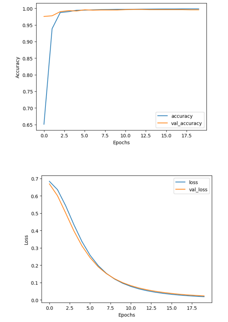
You can see that already after just a few epochs the model reached very high accuracy on both sets. But if you zoom in, you can see that the performance was still slightly improving on the training set through all 20 epochs, while it stagnated a bit earlier on the validation set. The loss on the other hand kept decreasing through all 20 epochs, which means that the model also got more confident in its predictions.
4.1 - Predict on Data
Now you can use the model for predictions on unseen tweets as model.predict(). This is as simple as passing an array of sequences you want to predict to the mentioned method.
In the cell below you prepare an extract of positive and negative samples from the validation set (remember, the positive examples are at the beginning and the negative are at the end) for the demonstration and predict their values with the model. Note that in the ideal case you should have another test set from which you would draw this data to inspect the model performance. But for the demonstration here the validation set will do just as well.
# Prepare an example with 10 positive and 10 negative tweets.
example_for_prediction = np.append(val_x_prepared[0:10], val_x_prepared[-10:], axis=0)

# Make a prediction on the tweets.
model.predict(example_for_prediction)
Output
1/1 [==============================] - 0s 67ms/step
Out[40]:
array([[0.9001521 ],
       [0.99429554],
       [0.99702805],
       [0.9513193 ],
       [0.9976744 ],
       [0.9960562 ],
       [0.9919789 ],
       [0.9800092 ],
       [0.9984914 ],
       [0.9983236 ],
       [0.01062678],
       [0.04205199],
       [0.01288154],
       [0.0168143 ],
       [0.01739226],
       [0.00625729],
       [0.01589022],
       [0.00809518],
       [0.02305534],
       [0.03285299]], dtype=float32)
You can see that the first 10 numbers are very close to 1, which means the model correctly predicted positive sentiment and the last 10 numbers are all close to zero, which means the model correctly predicted negative sentiment.
5 - Test With Your Own Input
Finally you will test with your own input. You will see that deepnets are more powerful than the older methods you have used before. Although you go close to 100 % accuracy on the first two assignments, you can see even more improvement here.
5.1 - Create the Prediction Function
def get_prediction_from_tweet(tweet, model, vocab, max_len):
    tweet = process_tweet(tweet)
    tweet = padded_sequence(tweet, vocab, max_len)
    tweet = np.array([tweet])

    prediction = model.predict(tweet, verbose=False)

    return prediction[0][0]
Now you can write your own tweet and see how the model predicts it. Try playing around with the words - for example change gr8 for great in the sample tweet and see if the score gets higher or lower.
Also Try writing your own tweet and see if you can find what affects the output most.
unseen_tweet = '@DLAI @NLP_team_dlai OMG!!! what a daaay, wow, wow. This AsSiGnMeNt was gr8.'

prediction_unseen = get_prediction_from_tweet(unseen_tweet, model, vocab, max_len)
print(f"Model prediction on unseen tweet: {prediction_unseen}")
Output
Model prediction on unseen tweet: 0.7467308640480042
Exercise 8 - graded_very_positive_tweet
Instructions: For your last exercise in this assignment, you need to write a very positive tweet. To pass this exercise, the tweet needs to score at least 0.99 with the model (which means the model thinks it is very positive).
Hint: try some positive words and/or happy smiley faces 😃
# GRADED VARIABLE: graded_very_positive_tweet

### START CODE HERE ###

# Please replace this sad tweet with a happier tweet
graded_very_positive_tweet = 'It is a very nice movie. Very happy to see it, great, excellent, best, good, better movie.'

### END CODE HERE ###
# Test your graded_very_positive_tweet tweet
prediction = get_prediction_from_tweet(graded_very_positive_tweet, model, vocab, max_len)
if prediction > 0.99:
    print("\033[92m All tests passed")
else:
    print("The model thinks your tweet is not positive enough.\nTry figuring out what makes some of the tweets in the validation set so positive.")
Output
All tests passed
6 - Word Embeddings
In this last section, you will visualize the word embeddings that your model has learned for this sentiment analysis task.
By using model.layers, you get a list of the layers in the model. The embeddings are saved in the first layer of the model (position 0).
You can retrieve the weights of the layer by calling layer.get_weights() function, which gives you a list of matrices with weights. The embedding layer has only one matrix in it, which contains your embeddings. Let’s extract the embeddings.
# Get the embedding layer
embeddings_layer = model.layers[0]

# Get the weights of the embedding layer
embeddings = embeddings_layer.get_weights()[0]

print(f"Weights of embedding layer have shape: {embeddings.shape}")
Output
Weights of embedding layer have shape: (9535, 16)
Since your embeddings are 16-dimensional (or different if you chose some other dimension), it is hard to visualize them without some kind of transformation. Here, you’ll use scikit-learn to perform dimensionality reduction of the word embeddings using PCA, with which you can reduce the number of dimensions to two, while keeping as much information as possible. Then you can visualize the data to see how the vectors for different words look like.
# PCA with two dimensions
pca = PCA(n_components=2)

# Dimensionality reduction of the word embeddings
embeddings_2D = pca.fit_transform(embeddings)
Now, everything is ready to plot a selection of words in 2d. Dont mind the axes on the plot - they point in the directions calculated by the PCA algorithm. Pay attention to which words group together.
#Selection of negative and positive words
neg_words = ['bad', 'hurt', 'sad', 'hate', 'worst']
pos_words = ['best', 'good', 'nice', 'love', 'better', ':)']

#Index of each selected word
neg_n = [vocab[w] for w in neg_words]
pos_n = [vocab[w] for w in pos_words]

plt.figure()

#Scatter plot for negative words
plt.scatter(embeddings_2D[neg_n][:,0], embeddings_2D[neg_n][:,1], color = 'r')
for i, txt in enumerate(neg_words):
    plt.annotate(txt, (embeddings_2D[neg_n][i,0], embeddings_2D[neg_n][i,1]))

#Scatter plot for positive words
plt.scatter(embeddings_2D[pos_n][:,0], embeddings_2D[pos_n][:,1], color = 'g')
for i, txt in enumerate(pos_words):
    plt.annotate(txt,(embeddings_2D[pos_n][i,0], embeddings_2D[pos_n][i,1]))

plt.title('Word embeddings in 2d')

plt.show()
Output
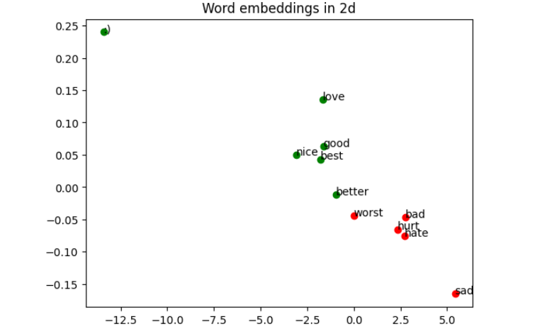
As you can see, the word embeddings for this task seem to distinguish negative and positive meanings. However, similar words don’t necessarily cluster together, since you only trained the model to analyze the overall sentiment. Notice how the smiley face is much further away from the negative words than any of the positive words are. It turns out that smiley faces are actually the most important predictors of sentiment in this dataset. Try removing them from the tweets (and consequently from the vocabulary) and see how well the model performs then. You should see quite a significant drop in performance.
Congratulations on finishing this assignment!
During this assignment you tested your theoretical and practical skills by creating a vocabulary of words in the tweets and coding a neural network that created word embeddings and classified the tweets into positive or negative. Next week you will start coding some sequence models!
Keep up the good work!
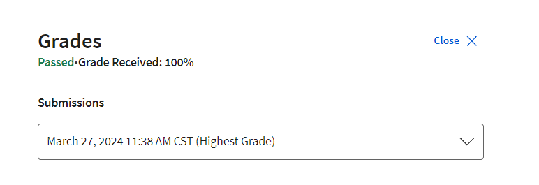
Grades
N-grams vs. Sequence Models
Traditional Language models
Traditional language models make use of probabilities to help identify which sentence is most likely to take place.
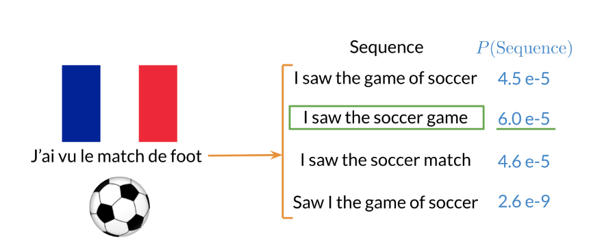
In the example above, the second sentence is the one that is most likely to take place as it has the highest probability of happening. To compute the probabilities, you can do the following:
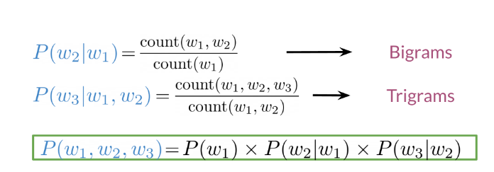
Large N-grams capture dependencies between distant words and need a lot of space and RAM. Hence, we resort to using different types of alternatives.
Recurrent Neural Networks
Previously, we tried using traditional language models, but it turns out they took a lot of space and RAM. For example, in the sentence below:
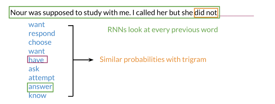
An N-gram (trigram) would only look at “did not” and would try to complete the sentence from there. As a result, the model will not be able to see the beginning of the sentence “I called her but she”. Probably the most likely word is have after “did not”. RNNs help us solve this problem by being able to track dependencies that are much further apart from each other. As the RNN makes its way through a text corpus, it picks up some information as follows:
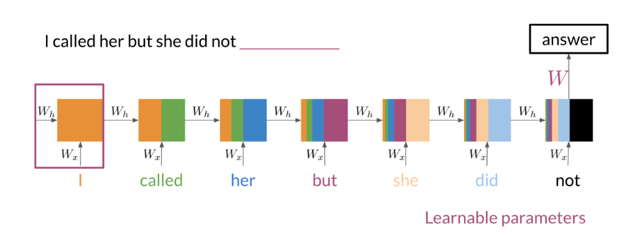
Note that as you feed in more information into the model, the previous word’s retention gets weaker, but it is still there. Look at the orange rectangle above and see how it becomes smaller as you make your way through the text. This shows that your model is capable of capturing dependencies and remembers a previous word although it is at the beginning of a sentence or paragraph. Another advantage of RNNs is that a lot of the computation shares parameters.
Application of RNNs
RNNs could be used in a variety of tasks ranging from machine translation to caption generation. There are many ways to implement an RNN model:
- One to One: given some scores of a championship, you can predict the winner.
- One to Many: given an image, you can predict what the caption is going to be.
- Many to One: given a tweet, you can predict the sentiment of that tweet.
- Many to Many: given an english sentence, you can translate it to its German equivalent.
In the next video, you will see the math in simple RNNs.
Math in Simple RNNs
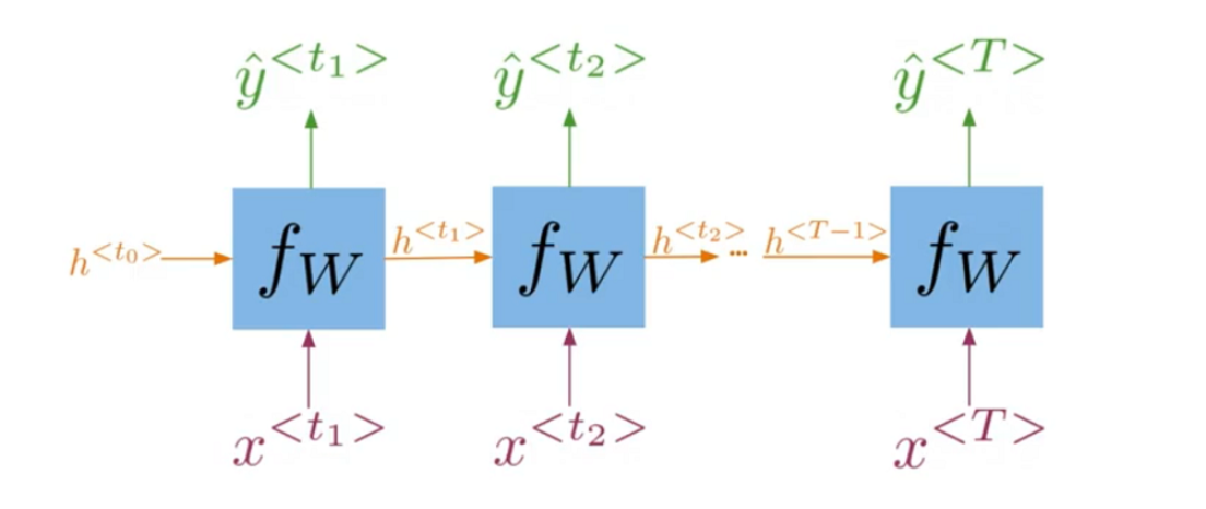
It is best to explain the math behind a simple RNN with a diagram:
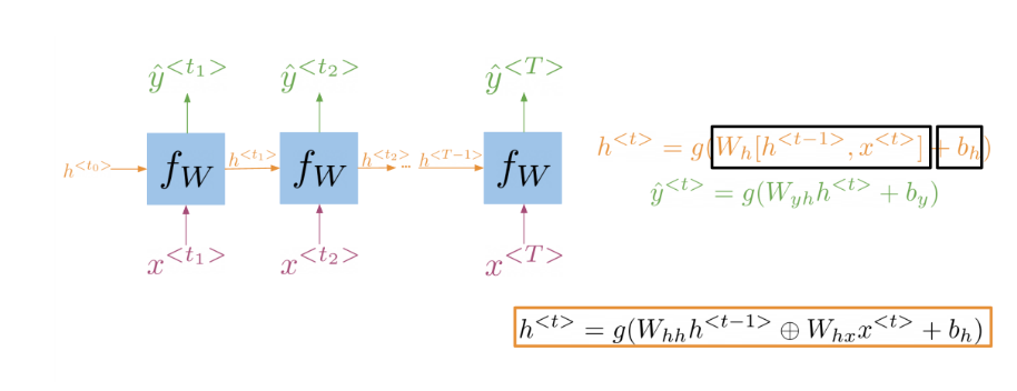
Note that:
h < t > = g ( W h [ h < t − 1 > , x < t > ] + b h ) h^{<t>}=g\bigl(W_{h}\bigl[h^{<t-1>},x^{<t>}\bigr]+b_{h}\bigr) h<t>=g(Wh[h<t−1>,x<t>]+bh)
Is the same as multiplying W h h W_{hh} Whh by h and W h x W_{hx} Whx by x. In other words, you can concatenate it as follows:
h < t > = g ( W h h h < t − 1 > ⊕ W h x x < t > + b h ) h^{<t>}=g\left(W_{hh}h^{<t-1>}\oplus W_{hx}x^{<t>}+b_h\right) h<t>=g(Whhh<t−1>⊕Whxx<t>+bh)
For the prediction at each time step, you can use thc following:
y ^ < t > = g ( W y h h < t > + b y ) \hat{y}^{<t>}=g\left(W_{yh}h^{<t>}+b_y\right) y^<t>=g(Wyhh<t>+by)
Note that you end up training W h h , W h x , W y h , b h , b y . W_{hh},W_{hx},W_{yh},b_h,b_y. Whh,Whx,Wyh,bh,by. Here is a visualization of the model.
Lab: Hidden State Activation
Hidden State Activation : Ungraded Lecture Notebook
In this notebook you’ll take another look at the hidden state activation function. It can be written in two different ways.
You will see, step by step, how to implement each of them and then how to verify whether the results produced by each of them are the same.
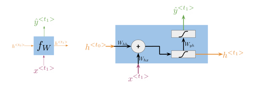
Background
Here you can see an image of a recurrent neural network (RNN). The hidden state activation function for a vanilla RNN can be written as an equation in two ways. You can either write it like this:
h < t > = g ( W h [ h < t − 1 > , x < t > ] + b h ) h^{<t>}=g(W_{h}[h^{<t-1>},x^{<t>}] + b_h) h<t>=g(Wh[h<t−1>,x<t>]+bh)
Or you can write it like this:
h < t > = g ( W h h h < t − 1 > + W h x x < t > + b h ) h^{<t>}=g(W_{hh}h^{<t-1>} + W_{hx}x^{<t>} + b_h) h<t>=g(Whhh<t−1>+Whxx<t>+bh)
The difference between the formulas is that in the first case you concatenate the matrices together and perform the multiplication only once, while in the second case you perform two separate multiplications and then sum them. More specifically:
W h W_{h} Wh in the first formula denotes the horizontal concatenation of weight matrices W h h W_{hh} Whh and W h x W_{hx} Whx from the second formula.
W h W_{h} Wh in the first formula is then multiplied by [ h < t − 1 > , x < t > ] [h^{<t-1>}, x^{<t>}] [h<t−1>,x<t>], another concatenation of parameters from the second formula but this time in a different direction, i.e vertical! In the second formula the two (non-concatenated) matrices are multiplied by its own respective parameter vector.
Below, you will calculate both options using NumPy
Imports
import numpy as np
Joining (Concatenation)
Weights
A join along the vertical boundary is called a horizontal concatenation or horizontal stack.
Visually, it looks like this:- W h = [ W h h ∣ W h x ] W_h = \left [ W_{hh} \ | \ W_{hx} \right ] Wh=[Whh ∣ Whx]
You will see two different ways to achieve this using numpy.
Note: The values used to populate the arrays, below, have been chosen to aid in visual illustration only. They are NOT what you’d expect to use building a model, which would typically be random variables instead.
- Try using random initializations for the weight arrays.
# Create some dummy data

w_hh = np.full((3, 2), 1)  # illustration purposes only, returns an array of size 3x2 filled with all 1s
w_hx = np.full((3, 3), 9)  # illustration purposes only, returns an array of size 3x3 filled with all 9s


### START CODE HERE ###
# Try using some random initializations, though it will obfuscate the join. eg: uncomment these lines
# w_hh = np.random.standard_normal((3,2))
# w_hx = np.random.standard_normal((3,3))
### END CODE HERE ###

print("-- Data --\n")
print("w_hh :")
print(w_hh)
print("w_hh shape :", w_hh.shape, "\n")
print("w_hx :")
print(w_hx)
print("w_hx shape :", w_hx.shape, "\n")

# Joining the arrays
print("-- Joining --\n")
# Option 1: concatenate - horizontal
w_h1 = np.concatenate((w_hh, w_hx), axis=1)
print("option 1 : concatenate\n")
print("w_h :")
print(w_h1)
print("w_h shape :", w_h1.shape, "\n")

# Option 2: hstack
w_h2 = np.hstack((w_hh, w_hx))
print("option 2 : hstack\n")
print("w_h :")
print(w_h2)
print("w_h shape :", w_h2.shape)
Output
-- Data --

w_hh :
[[1 1]
 [1 1]
 [1 1]]
w_hh shape : (3, 2)

w_hx :
[[9 9 9]
 [9 9 9]
 [9 9 9]]
w_hx shape : (3, 3)

-- Joining --

option 1 : concatenate

w_h :
[[1 1 9 9 9]
 [1 1 9 9 9]
 [1 1 9 9 9]]
w_h shape : (3, 5)

option 2 : hstack

w_h :
[[1 1 9 9 9]
 [1 1 9 9 9]
 [1 1 9 9 9]]
w_h shape : (3, 5)
Hidden State & Inputs
Joining along a horizontal boundary is called a vertical concatenation or vertical stack. Visually it looks like this:
[ h < t − 1 > , x < t > ] = [ h < t − 1 > x < t > ] [h^{<t-1>},x^{<t>}] = \left[ \frac{h^{<t-1>}}{x^{<t>}} \right] [h<t−1>,x<t>]=[x<t>h<t−1>]
You will see two different ways to achieve this using numpy.
Try using random initializations for the hidden state and input matrices.
# Create some more dummy data
h_t_prev = np.full((2, 1), 1)  # illustration purposes only, returns an array of size 2x1 filled with all 1s
x_t = np.full((3, 1), 9)       # illustration purposes only, returns an array of size 3x1 filled with all 9s

# Try using some random initializations, though it will obfuscate the join. eg: uncomment these lines

### START CODE HERE ###
# h_t_prev = np.random.standard_normal((2,1))
# x_t = np.random.standard_normal((3,1))
### END CODE HERE ###

print("-- Data --\n")
print("h_t_prev :")
print(h_t_prev)
print("h_t_prev shape :", h_t_prev.shape, "\n")
print("x_t :")
print(x_t)
print("x_t shape :", x_t.shape, "\n")

# Joining the arrays
print("-- Joining --\n")

# Option 1: concatenate - vertical
ax_1 = np.concatenate(
    (h_t_prev, x_t), axis=0
)  # note the difference in axis parameter vs earlier
print("option 1 : concatenate\n")
print("ax_1 :")
print(ax_1)
print("ax_1 shape :", ax_1.shape, "\n")

# Option 2: vstack
ax_2 = np.vstack((h_t_prev, x_t))
print("option 2 : vstack\n")
print("ax_2 :")
print(ax_2)
print("ax_2 shape :", ax_2.shape)
Output
-- Data --

h_t_prev :
[[1]
 [1]]
h_t_prev shape : (2, 1)

x_t :
[[9]
 [9]
 [9]]
x_t shape : (3, 1)

-- Joining --

option 1 : concatenate

ax_1 :
[[1]
 [1]
 [9]
 [9]
 [9]]
ax_1 shape : (5, 1)

option 2 : vstack

ax_2 :
[[1]
 [1]
 [9]
 [9]
 [9]]
ax_2 shape : (5, 1)
Verify Formulas
Now you know how to do the concatenations, horizontal and vertical, lets verify if the two formulas produce the same result.
Formula 1: h < t > = g ( W h [ h < t − 1 > , x < t > ] + b h ) h^{<t>}=g(W_{h}[h^{<t-1>},x^{<t>}] + b_h) h<t>=g(Wh[h<t−1>,x<t>]+bh)
Formula 2: h < t > = g ( W h h h < t − 1 > + W h x x < t > + b h ) h^{<t>}=g(W_{hh}h^{<t-1>} + W_{hx}x^{<t>} + b_h) h<t>=g(Whhh<t−1>+Whxx<t>+bh)
To prove: Formula 1 ⇔ \Leftrightarrow ⇔ Formula 2
You will ignore the bias term b h b_h bh and the activation function g ( ) g(\ ) g( ) because the transformation will be identical for each formula. So what we really want to compare is the result of the following parameters inside each formula:
$W_{h}[h{<t-1>},x{}] \quad \Leftrightarrow \quad W_{hh}h^{} + W_{hx}x^{} $
You will do this by using matrix multiplication combined with the data and techniques (stacking/concatenating) from above.
- Try adding a sigmoid activation function and bias term to the checks for completeness.
# Data

w_hh = np.full((3, 2), 1)  # returns an array of size 3x2 filled with all 1s
w_hx = np.full((3, 3), 9)  # returns an array of size 3x3 filled with all 9s
h_t_prev = np.full((2, 1), 1)  # returns an array of size 2x1 filled with all 1s
x_t = np.full((3, 1), 9)       # returns an array of size 3x1 filled with all 9s


# If you want to randomize the values, uncomment the next 4 lines

# w_hh = np.random.standard_normal((3,2))
# w_hx = np.random.standard_normal((3,3))
# h_t_prev = np.random.standard_normal((2,1))
# x_t = np.random.standard_normal((3,1))

# Results
print("-- Results --")
# Formula 1
stack_1 = np.hstack((w_hh, w_hx))
stack_2 = np.vstack((h_t_prev, x_t))

print("\nFormula 1")
print("Term1:\n",stack_1)
print("Term2:\n",stack_2)
formula_1 = np.matmul(np.hstack((w_hh, w_hx)), np.vstack((h_t_prev, x_t)))
print("Output:")
print(formula_1)

# Formula 2
mul_1 = np.matmul(w_hh, h_t_prev)
mul_2 = np.matmul(w_hx, x_t)
print("\nFormula 2")
print("Term1:\n",mul_1)
print("Term2:\n",mul_2)

formula_2 = np.matmul(w_hh, h_t_prev) + np.matmul(w_hx, x_t)
print("\nOutput:")
print(formula_2, "\n")

# Verification
# np.allclose - to check if two arrays are elementwise equal upto certain tolerance, here
# https://numpy.org/doc/stable/reference/generated/numpy.allclose.html

print("-- Verify --")
print("Results are the same :", np.allclose(formula_1, formula_2))

### START CODE HERE ###
# # Try adding a sigmoid activation function and bias term as a final check
# # Activation
# def sigmoid(x):
#     return 1 / (1 + np.exp(-x))

# # Bias and check
# b = np.random.standard_normal((formula_1.shape[0],1))
# print("Formula 1 Output:\n",sigmoid(formula_1+b))
# print("Formula 2 Output:\n",sigmoid(formula_2+b))

# all_close = np.allclose(sigmoid(formula_1+b), sigmoid(formula_2+b))
# print("Results after activation are the same :",all_close)
### END CODE HERE ###
Output
-- Results --

Formula 1
Term1:
 [[1 1 9 9 9]
 [1 1 9 9 9]
 [1 1 9 9 9]]
Term2:
 [[1]
 [1]
 [9]
 [9]
 [9]]
Output:
[[245]
 [245]
 [245]]

Formula 2
Term1:
 [[2]
 [2]
 [2]]
Term2:
 [[243]
 [243]
 [243]]

Output:
[[245]
 [245]
 [245]]

-- Verify --
Results are the same : True
Summary
That’s it! You have verified that the two formulas produce the same results, and seen how to combine matrices vertically and horizontally to make that happen. You now have all the intuition needed to understand the math notation of RNNs.
Cost Function for RNNs
The cost function used in an RNN is the cross entropy loss. If you were to visualize it
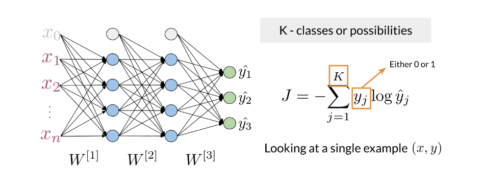
you are basically summing over the all the classes and then multiplying y j y_j yj times log y ^ j \log\hat{y}_j logy^j. If you were to compute the loss over several time steps, use the following formula:
J = − 1 T ∑ t = 1 T ∑ j = 1 K y j < t > log y ^ j < t > J=-\frac{1}{T}\sum_{t=1}^{T}\sum_{j=1}^{K}y_{j}^{<t>}\log\hat{y}_{j}^{<t>} J=−T1t=1∑Tj=1∑Kyj<t>logy^j<t>
Note that we are simply summing over all the time steps and dividing by T, to get the average cost in each time step. Hence, we are just taking an average through time.
Implementation Note
The scan function is built as follows:
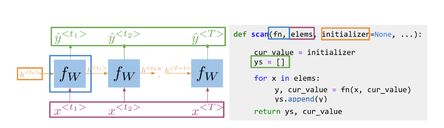
Note, that is basically what an RNN is doing. It takes the initializer, and returns a list of outputs (ys), and uses the current value, to get the next y and the next current value. These type of abstractions allow for much faster computation.
Gated Recurrent Units
Gated recurrent units are very similar to vanilla RNNs, except that they have a “relevance” and “update” gate that allow the model to update and get relevant information. I personally find it easier to understand by looking at the formulas:
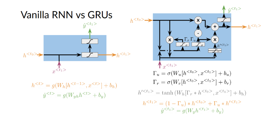
To the left, you have the diagram and equations for a simple RNN. To the right, we explain the GRU. Note that we add 3 layers before computing h and y.
Γ u = σ ( W u [ h < t 0 > , x < t 1 > ] + b u ) Γ r = σ ( W r [ h < t 0 > , x < t 1 > ] + b r ) h ′ < t 1 > = tanh ( W h [ Γ r ∗ h < t 0 > , x < t 1 > ] + b h ) \begin{aligned}\Gamma_u&=\sigma\left(W_u\left[h^{<t_0>},x^{<t_1>}\right]+b_u\right)\\\Gamma_r&=\sigma\left(W_r\left[h^{<t_0>},x^{<t_1>}\right]+b_r\right)\\h^{\prime<t_1>}&=\tanh\left(W_h\left[\Gamma_r*h^{<t_0>},x^{<t_1>}\right]+b_h\right)\end{aligned} ΓuΓrh′<t1>=σ(Wu[h<t0>,x<t1>]+bu)=σ(Wr[h<t0>,x<t1>]+br)=tanh(Wh[Γr∗h<t0>,x<t1>]+bh)
Thefirst gate Γ u \Gamma_u Γu allows you to decide how much you want to update the weights by. The second gate Γ r \Gamma_{r} Γr, helps you find a relevance score. You can compute the new h h h by using the relevance gate. Finally you can compute h h h, using the update gate. GRUs“decide” how to update the hidden state. GRUs help preserve important information.
Lab: Vanilla RNNs, GRUs and the scan function
In this notebook, you will learn how to define the forward method for vanilla RNNs and GRUs from scratch in NumPy. After this, you will create a full neural network with GRU layers using tensorflow.
By completing this notebook, you will:
- Be able to define the forward method for vanilla RNNs and GRUs
- Be able to build a sequential model using recurrent layers in tensorflow
- Be able to use the
return_sequencesparameter in recurrent layers
import numpy as np
from numpy import random
from time import perf_counter
import tensorflow as tf
An implementation of the sigmoid function is provided below so you can use it in this notebook.
def sigmoid(x): # Sigmoid function
    return 1.0 / (1.0 + np.exp(-x))
Part 1: Forward method for vanilla RNNs and GRUs using numpy
In this part of the notebook, you’ll see the implementation of the forward method for a vanilla RNN and you’ll implement that same method for a GRU. For this exercise you’ll use a set of random weights and variables with the following dimensions:
- Embedding size (
emb) : 128 - Hidden state size (
h_dim) : 16
The weights w_ and biases b_ are initialized with dimensions (h_dim, emb + h_dim) and (h_dim, 1). We expect the hidden state h_t to be a column vector with size (h_dim,1) and the initial hidden state h_0 is a vector of zeros.
random.seed(10)                 # Random seed, so your results match ours
emb = 128                       # Embedding size
T = 256                         # Length of sequence
h_dim = 16                      # Hidden state dimension
h_0 = np.zeros((h_dim, 1))      # Initial hidden state

# Random initialization of weights (w1, w2, w3) and biases (b1, b2, b3)
w1 = random.standard_normal((h_dim, emb + h_dim))
w2 = random.standard_normal((h_dim, emb + h_dim))
w3 = random.standard_normal((h_dim, emb + h_dim))
b1 = random.standard_normal((h_dim, 1))
b2 = random.standard_normal((h_dim, 1))
b3 = random.standard_normal((h_dim, 1))
# Random initialization of input X
# Note that you add the third dimension (1) to achieve the batch representation.
X = random.standard_normal((T, emb, 1))

# Define the lists of weights as you will need them for the two different layers
weights_vanilla = [w1, b1]
weights_GRU = [w1.copy(), w2, w3, b1.copy(), b2, b3]
Note that you are creating two lists where you are storing all the weights. You can see that the vanilla recurrent neural network uses a much smaller subset of weights than GRU. Since you will not be updating any weights in this lab, it is ok to define them in a list like above.
1.1 Forward method for vanilla RNNs
The vanilla RNN cell is quite straight forward. Its most general structure is presented in the next figure:
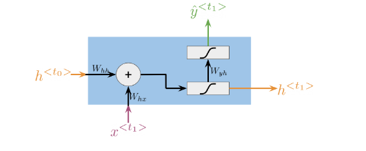
As you saw in the lecture videos and in the other lab, the computations made in a vanilla RNN cell are equivalent to the following equations:
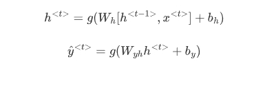
where [ h < t − 1 > , x < t > ] [h^{<t-1>},x^{<t>}] [h<t−1>,x<t>] means that h < t − 1 > h^{<t-1>} h<t−1> and x < t > x^{<t>} x<t> are concatenated together. In the next cell you have the implementation of the forward method for a vanilla RNN.
def forward_V_RNN(inputs, weights): # Forward propagation for a a single vanilla RNN cell
    x, h_t = inputs

    # weights.
    wh, bh = weights

    # new hidden state
    h_t = np.dot(wh, np.concatenate([h_t, x])) + bh
    h_t = sigmoid(h_t)

    # We avoid implementation of y for clarity
    y = h_t

    return y, h_t
As you can see, we omitted the computation of y ^ < t > \hat{y}^{<t>} y^<t>. This was done for the sake of simplicity, so you can focus on the way that hidden states are updated here and in the GRU cell.
1.2 Forward method for GRUs
A GRU cell has many more computations than vanilla RNN cells. You can see this visually in the following diagram:
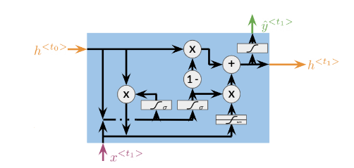
As you saw in the lecture videos, GRUs have relevance Γ r \Gamma_r Γr and update Γ u \Gamma_u Γu gates that control how the hidden state h < t > h^{<t>} h<t> is updated on every time step. With these gates, GRUs are capable of keeping relevant information in the hidden state even for long sequences. The equations needed for the forward method in GRUs are provided below:
Γ r = σ ( W r [ h < t − 1 > , x < t > ] + b r ) \begin{equation} \Gamma_r=\sigma{(W_r[h^{<t-1>}, x^{<t>}]+b_r)} \end{equation} Γr=σ(Wr[h<t−1>,x<t>]+br)
Γ u = σ ( W u [ h < t − 1 > , x < t > ] + b u ) \begin{equation} \Gamma_u=\sigma{(W_u[h^{<t-1>}, x^{<t>}]+b_u)} \end{equation} Γu=σ(Wu[h<t−1>,x<t>]+bu)
c < t > = tanh ( W h [ Γ r ∗ h < t − 1 > , x < t > ] + b h ) \begin{equation} c^{<t>}=\tanh{(W_h[\Gamma_r*h^{<t-1>},x^{<t>}]+b_h)} \end{equation} c<t>=tanh(Wh[Γr∗h<t−1>,x<t>]+bh)
h < t > = Γ u ∗ c < t > + ( 1 − Γ u ) ∗ h < t − 1 > \begin{equation} h^{<t>}=\Gamma_u*c^{<t>}+(1-\Gamma_u)*h^{<t-1>} \end{equation} h<t>=Γu∗c<t>+(1−Γu)∗h<t−1>
In the next cell, you will see the implementation of the forward method for a GRU cell by computing the update u and relevance r gates, and the candidate hidden state c.
def forward_GRU(inputs, weights): # Forward propagation for a single GRU cell
    x, h_t = inputs

    # weights.
    wu, wr, wc, bu, br, bc = weights

    # Update gate
    u = np.dot(wu, np.concatenate([h_t, x])) + bu
    u = sigmoid(u)

    # Relevance gate
    r = np.dot(wr, np.concatenate([h_t, x])) + br
    r = sigmoid(r)

    # Candidate hidden state
    c = np.dot(wc, np.concatenate([r * h_t, x])) + bc
    c = np.tanh(c)

    # New Hidden state h_t
    h_t = u * c + (1 - u) * h_t

    # We avoid implementation of y for clarity
    y = h_t

    return y, h_t
Run the following cell to check your implementation.
forward_GRU([X[1], h_0], weights_GRU)[0]
Output
array([[ 9.77779014e-01],
       [-9.97986240e-01],
       [-5.19958083e-01],
       [-9.99999886e-01],
       [-9.99707004e-01],
       [-3.02197037e-04],
       [-9.58733503e-01],
       [ 2.10804828e-02],
       [ 9.77365398e-05],
       [ 9.99833090e-01],
       [ 1.63200940e-08],
       [ 8.51874303e-01],
       [ 5.21399924e-02],
       [ 2.15495959e-02],
       [ 9.99878828e-01],
       [ 9.77165472e-01]])
Expected output:
array([[ 9.77779014e-01],
       [-9.97986240e-01],
       [-5.19958083e-01],
       [-9.99999886e-01],
       [-9.99707004e-01],
       [-3.02197037e-04],
       [-9.58733503e-01],
       [ 2.10804828e-02],
       [ 9.77365398e-05],
       [ 9.99833090e-01],
       [ 1.63200940e-08],
       [ 8.51874303e-01],
       [ 5.21399924e-02],
       [ 2.15495959e-02],
       [ 9.99878828e-01],
       [ 9.77165472e-01]])
1.3 Implementation of the scan function
In the lectures you saw how the scan function is used for forward propagation in RNNs. It takes as inputs:
fn: the function to be called recurrently (i.e.forward_GRU)elems: the list of inputs for each time step (X)weights: the parameters needed to computefnh_0: the initial hidden state
scan goes through all the elements x in elems, calls the function fn with arguments ([x, h_t],weights), stores the computed hidden state h_t and appends the result to a list ys. Complete the following cell by calling fn with arguments ([x, h_t],weights).
def scan(fn, elems, weights, h_0): # Forward propagation for RNNs
    h_t = h_0
    ys = []

    for x in elems:
        y, h_t = fn([x, h_t], weights)
        ys.append(y)

    return ys, h_t
In practice, when using libraries like TensorFlow you don’t need to use functions like scan, because this is already implemented under the hood for you. But it is still useful to understand it as you may need to code it from scratch at some point.
In the cell below, you can try the scan function on the data you created above with the function forward_V_RNN and see what it outputs.
ys, h_T = scan(forward_V_RNN, X, weights_vanilla, h_0)

print(f"Length of ys: {len(ys)}")
print(f"Shape of each y within ys: {ys[0].shape}")
print(f"Shape of h_T: {h_T.shape}")
Output
Length of ys: 256
Shape of each y within ys: (16, 1)
Shape of h_T: (16, 1)
You can see that it outputs a sequence of length 256, where each element in a sequence is the same shape as the hidden state (because that is how you defined your forward_V_RNN function).
1.4 Comparison between vanilla RNNs and GRUs
You have already seen how forward propagation is computed for vanilla RNNs and GRUs. As a quick recap, you need to have a forward method for the recurrent cell and a function like scan to go through all the elements from a sequence using a forward method. You saw that GRUs performed more computations than vanilla RNNs, and you can check that they have 3 times more parameters. In the next two cells, we compute forward propagation for a sequence with 256 time steps (T) for an RNN and a GRU with the same hidden state h_t size (h_dim=16).
# vanilla RNNs
tic = perf_counter()
ys, h_T = scan(forward_V_RNN, X, weights_vanilla, h_0)
toc = perf_counter()
RNN_time=(toc-tic)*1000
print (f"It took {RNN_time:.2f}ms to run the forward method for the vanilla RNN.")
Output
It took 3.56ms to run the forward method for the vanilla RNN.
# GRUs
tic = perf_counter()
ys, h_T = scan(forward_GRU, X, weights_GRU, h_0)
toc = perf_counter()
GRU_time=(toc-tic)*1000
print (f"It took {GRU_time:.2f}ms to run the forward method for the GRU.")
Output
It took 9.25ms to run the forward method for the GRU.
As you saw in the lectures, GRUs take more time to compute. This means that training and prediction would take more time for a GRU than for a vanilla RNN. However, GRUs allow you to propagate relevant information even for long sequences, so when selecting an architecture for NLP you should assess the tradeoff between computational time and performance.
Part 2: Create a GRU model in tensorflow
You will use the Sequential model using some GRU layers. You should already be familiar with the sequential model and with the Dense layers. In addition, you will use GRU layers in this notebook. Below you can find some links to the documentation and a short description.
SequentialA Sequential model is appropriate for a plain stack of layers where each layer has exactly one input tensor and one output tensor.DenseA regular fully connected layerGRUThe GRU (gated recurrent unit) layer. The hidden state dimension should be specified (the syntax is the same as forDense). By default it does not return a sequence, but only the output of the last unit. If you want to stack two consecutive GRU layers, you need the first one to output a sequence, which you can achieve by setting the parameterreturn_sequencesto True. If you are further interested in similar layers, you can also check out theRNN,LSTMandBidirectional. If you want to use a RNN or LSTM instead of GRU in the code below, simply change the layer name, no other change in the syntax is needed.
Putting everything together the GRU model will look like this:
model_GRU = tf.keras.Sequential([
    tf.keras.layers.GRU(256, return_sequences=True, name='GRU_1_returns_seq'),
    tf.keras.layers.GRU(128, return_sequences=True, name='GRU_2_returns_seq'),
    tf.keras.layers.GRU(64, name='GRU_3_returns_last_only'),
    tf.keras.layers.Dense(10)
])
To see how your model looks like, you can print out its summary. But beware, you cannot look at model’s summary before the model knows what kind of data it should expect.
# This line should fail
try:
    model_GRU.summary()
except Exception as e:
    print(e)
Output
This model has not yet been built. Build the model first by calling `build()` or by calling the model on a batch of data.
You see that the exception says that the model has not yet been built, so it does not allow you to see its summary. You will see two options on how to build a model that are described in the exception above.
First, you will define some input data (a random tensor) of the desired shape and pass this data through the model. Now the model knows the shape of the data and can also calculate the number of parameters it needs for each layer, so the .summary() method should work.
# Remember these three numbers and follow them further through the notebook
batch_size = 60
sequence_length = 50
word_vector_length = 40

input_data = tf.random.normal([batch_size, sequence_length, word_vector_length])

# Pass the data through the network
prediction = model_GRU(input_data)

# Show the summary of the model
model_GRU.summary()
Output
Model: "sequential"
_________________________________________________________________
 Layer (type)                Output Shape              Param #
=================================================================
 GRU_1_returns_seq (GRU)     (60, 50, 256)             228864

 GRU_2_returns_seq (GRU)     (60, 50, 128)             148224

 GRU_3_returns_last_only (G  (60, 64)                  37248
 RU)

 dense (Dense)               (60, 10)                  650

=================================================================
Total params: 414986 (1.58 MB)
Trainable params: 414986 (1.58 MB)
Non-trainable params: 0 (0.00 Byte)
_________________________________________________________________
Now you can inspect the numbers in the Output Shape column. Note that all the numbers for parameters are distinct (each number is different), so you can more easily inspect what is going on (typically the batch size would be a power of 2, but here we choose it to be 60, just to be distinct from other numbers).
- You can see that the
word_vector_length(originally set to 40) which represents the word embedding dimension is already being changed to 256 in the first row. In other words, the model’s first GRU layer takes the original 40-dimensional word vectors and transforms them into its own 256-dimensional representations. - Next you can look at the
sequence_length(originally set to 50). The sequence length propagates through the model in the first two layers and then disappears. Note that these are the two GRU layers that return sequences, while the last GRU layer does not return a sequence, but only the output from the last cell, thus one dimension disappears from the model. - Lastly have a look at the
batch_size(originally set to 60), which propagates through the whole model (which makes sense, right?).
Now if you try to pass data of different shape through the network, it might be allowed in some cases, but not in others, let’s see this in action.
# Define some data with a different length of word vectors
new_word_vector_length = 44  # Before it was 40
# Keep the batch_size = 60 and sequence_length = 50 as originally
input_data_1 = tf.random.normal([batch_size, sequence_length, new_word_vector_length])

# Pass the data through the network. This should Fail (if you ran all the cells above)
try:
    prediction = model_GRU(input_data_1)
except Exception as e:
    print(e)
Output
Exception encountered when calling layer 'sequential' (type Sequential).

Input 0 of layer "GRU_1_returns_seq" is incompatible with the layer: expected shape=(None, None, 40), found shape=(60, 50, 44)

Call arguments received by layer 'sequential' (type Sequential):
  • inputs=tf.Tensor(shape=(60, 50, 44), dtype=float32)
  • training=None
  • mask=None
Why did this fail? Remember how the layers are constructed: they know what length of vectors to expect and they have their weight matrices defined to accommodate for it. However if you change the length of the word vector, it cannot be multiplied by an incompatible matrix .
How about the sequence_length (number of words)?
# Define some data with a different length of the sequence
new_sequence_length = 55  # Before it was 50
# Keep the batch_size = 60 and word_vector_length = 40 as originally
input_data_2 = tf.random.normal([batch_size, new_sequence_length, word_vector_length])

# Pass the data through the network. This should Fail (if you ran all the cells above)
prediction = model_GRU(input_data_2)

model_GRU.summary()
Output
Model: "sequential"
_________________________________________________________________
 Layer (type)                Output Shape              Param #
=================================================================
 GRU_1_returns_seq (GRU)     (60, None, 256)           228864

 GRU_2_returns_seq (GRU)     (60, None, 128)           148224

 GRU_3_returns_last_only (G  (60, 64)                  37248
 RU)

 dense (Dense)               (60, 10)                  650

=================================================================
Total params: 414986 (1.58 MB)
Trainable params: 414986 (1.58 MB)
Non-trainable params: 0 (0.00 Byte)
_________________________________________________________________
Well, this worked! Why? because the neural network does not have any specific parameters (weights) associated with the length of the sequence, so it is flexible in this dimension. Look at the summary at what happened in the second dimension of the output of the first two layers. Where there was “50” before, it turned to “None”. This tells you that the network now expects any sequence length.
How about batch_size? If you guessed it must also be flexible, you are right. You can any time change the batch size and the model should be fine with it. Let’s test it.
# Define some data with a different batch size
new_batch_size = 66  # Before it was 60
# Keep the sequence_length = 50 and word_vector_length = 40 as originally
input_data_3 = tf.random.normal([new_batch_size, sequence_length, word_vector_length])

# Pass the data through the network. This should Fail (if you ran all the cells above)
prediction = model_GRU(input_data_3)

model_GRU.summary()
Output
Model: "sequential"
_________________________________________________________________
 Layer (type)                Output Shape              Param #
=================================================================
 GRU_1_returns_seq (GRU)     (None, None, 256)         228864

 GRU_2_returns_seq (GRU)     (None, None, 128)         148224

 GRU_3_returns_last_only (G  (None, 64)                37248
 RU)

 dense (Dense)               (None, 10)                650

=================================================================
Total params: 414986 (1.58 MB)
Trainable params: 414986 (1.58 MB)
Non-trainable params: 0 (0.00 Byte)
_________________________________________________________________
Now the output shape has “None” everywhere except for the last dimension of each layer. This means it accepts batches and sequences of any size, but the length of the word vector and the hidden states stay the same.
Alternative: use model.build().
Rather than passing data through the model, you can also specify the size of the data in an array and pass it to model.build(). This will build the model, taking into account the data shape. You can also pass None, where the data dimension may change.
model_GRU_2 = tf.keras.Sequential([
    tf.keras.layers.GRU(256, return_sequences=True, name='GRU_1_returns_seq'),
    tf.keras.layers.GRU(128, return_sequences=True, name='GRU_2_returns_seq'),
    tf.keras.layers.GRU(64, name='GRU_3_returns_last_only'),
    tf.keras.layers.Dense(10)
])

model_GRU_2.build([None, None, word_vector_length])

model_GRU_2.summary()
Output
Model: "sequential_1"
_________________________________________________________________
 Layer (type)                Output Shape              Param #
=================================================================
 GRU_1_returns_seq (GRU)     (None, None, 256)         228864

 GRU_2_returns_seq (GRU)     (None, None, 128)         148224

 GRU_3_returns_last_only (G  (None, 64)                37248
 RU)

 dense_1 (Dense)             (None, 10)                650

=================================================================
Total params: 414986 (1.58 MB)
Trainable params: 414986 (1.58 MB)
Non-trainable params: 0 (0.00 Byte)
_________________________________________________________________
Congratulations! Now you know how the forward method is implemented for vanilla RNNs and GRUs, and you can implement them in tensorflow.
Deep and Bi-directional RNNs
Bi-directional RNNs are important, because knowing what is next in the sentence could give you more context about the sentence itself.
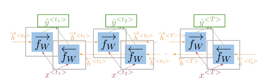
So you can see, in order to make a prediction y ^ \hat{y} y^, you will use the hidden states from both directions and combine them to make one hidden state, you can then proceed as you would with a simple vanilla RNN. When implementing Deep RNNs, you would compute the following.
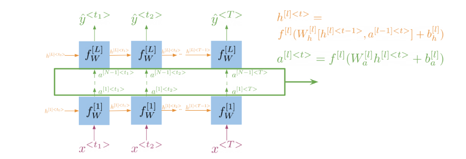
Note that at layer l l l, you are using the input from the bottom a [ l − 1 ] a^{[l-1]} a[l−1] and the hidden state h l h^l hl. That allows you to get your new h, and then to get your new a, you will train another weight matrix W a W_{a} Wa, which you will multiply by the corresponding h add the bias and then run it through an activation layer.
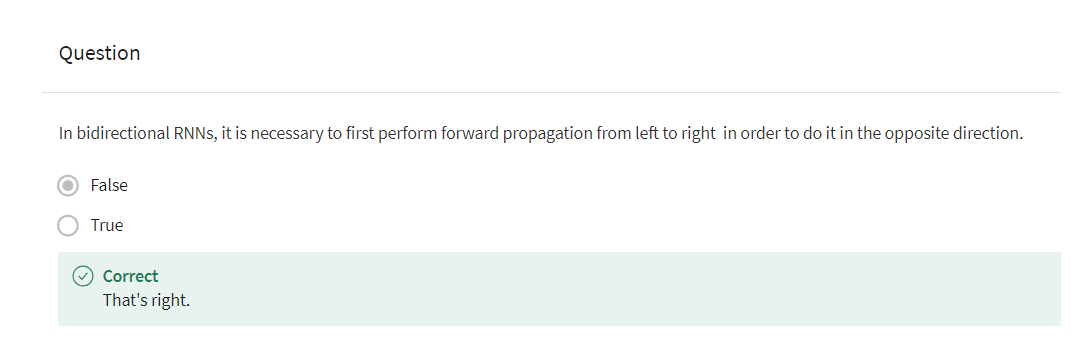
Lab: Calculating Perplexity
Calculating perplexity using numpy: Ungraded Lecture Notebook
In this notebook you will learn how to calculate perplexity. You will calculate it from scratch using numpy library. First you can import it and set the random seed, so that the results will be reproducible.
import numpy as np

# Setting random seeds
np.random.seed(32)
Calculating Perplexity
The perplexity is a metric that measures how well a probability model predicts a sample and it is commonly used to evaluate language models. It is defined as:
P ( W ) = ∏ i = 1 N 1 P ( w i ∣ w 1 , . . . , w i − 1 ) N P(W) = \sqrt[N]{\prod_{i=1}^{N} \frac{1}{P(w_i| w_1,...,w_{i-1})}} P(W)=Ni=1∏NP(wi∣w1,...,wi−1)1
Where P ( ) P() P() denotes probability and w i w_i wi denotes the i-th word, so P ( w i ∣ w 1 , . . . , w i − 1 ) P(w_i| w_1,...,w_{i-1}) P(wi∣w1,...,wi−1) is the probability of word i i i, given all previous words ( 1 1 1 to i − 1 i-1 i−1).
As an implementation hack, you would usually take the log of that formula (so the computation is less prone to underflow problems). You would also need to take care of the padding, since you do not want to include the padding when calculating the perplexity (to avoid an artificially good metric).
After taking the logarithm of P ( W ) P(W) P(W) you have:
l o g P ( W ) = log ( ∏ i = 1 N 1 P ( w i ∣ w 1 , . . . , w i − 1 ) N ) log P(W) = {\log\left(\sqrt[N]{\prod_{i=1}^{N} \frac{1}{P(w_i| w_1,...,w_{i-1})}}\right)} logP(W)=log Ni=1∏NP(wi∣w1,...,wi−1)1
= log ( ( ∏ i = 1 N 1 P ( w i ∣ w 1 , . . . , w i − 1 ) ) 1 N ) = \log\left(\left(\prod_{i=1}^{N} \frac{1}{P(w_i| w_1,...,w_{i-1})}\right)^{\frac{1}{N}}\right) =log (i=1∏NP(wi∣w1,...,wi−1)1)N1
= log ( ( ∏ i = 1 N P ( w i ∣ w 1 , . . . , w i − 1 ) ) − 1 N ) = \log\left(\left({\prod_{i=1}^{N}{P(w_i| w_1,...,w_{i-1})}}\right)^{-\frac{1}{N}}\right) =log (i=1∏NP(wi∣w1,...,wi−1))−N1
= − 1 N log ( ∏ i = 1 N P ( w i ∣ w 1 , . . . , w i − 1 ) ) = -\frac{1}{N}{\log\left({\prod_{i=1}^{N}{P(w_i| w_1,...,w_{i-1})}}\right)} =−N1log(i=1∏NP(wi∣w1,...,wi−1))
= − 1 N ∑ i = 1 N log P ( w i ∣ w 1 , . . . , w i − 1 ) = -\frac{1}{N}{{\sum_{i=1}^{N}{\log P(w_i| w_1,...,w_{i-1})}}} =−N1i=1∑NlogP(wi∣w1,...,wi−1)
You will be working with a real example from this week’s assignment. The example is made up of:
predictions: log probabilities for each element in the vocabulary for 32 sequences with 64 elements (after padding).targets: 32 observed sequences of 64 elements (after padding).
# Load from .npy files
predictions = np.load('predictions.npy')
targets = np.load('targets.npy')

# Print shapes
print(f'predictions has shape: {predictions.shape}')
print(f'targets has shape: {targets.shape}')
Output
predictions has shape: (32, 64, 256)
targets has shape: (32, 64)
Notice that the predictions have an extra dimension with the same length as the size of the vocabulary used.
Because of this you will need a way of reshaping targets to match this shape. For this you can use np.eye(), which you can use to create one-hot vectors.
Notice that predictions.shape[-1] will return the size of the last dimension of predictions.
reshaped_targets = np.eye(predictions.shape[-1])[targets]
print(f'reshaped_targets has shape: {reshaped_targets.shape}')
Output
reshaped_targets has shape: (32, 64, 256)
By calculating the product of the predictions and the reshaped targets and summing across the last dimension, the total log probability of each observed element within the sequences can be computed:
log_p = np.sum(predictions * reshaped_targets, axis= -1)
Now you will need to account for the padding so this metric is not artificially deflated (since a lower perplexity means a better model). For identifying which elements are padding and which are not, you can use np.equal() and get a tensor with 1s in the positions of actual values and 0s where there are paddings.
non_pad = 1.0 - np.equal(targets, 0)
print(f'non_pad has shape: {non_pad.shape}\n')
print(f'non_pad looks like this: \n\n {non_pad}')
这行代码的作用是根据 targets 数组中是否为零来创建一个新的数组 non_pad,其中非零元素对应的位置值为 1.0,而零元素对应的位置值为 0.0。
具体解释如下:
np.equal(targets, 0):这一部分先创建一个与targets数组相同大小的布尔类型的数组,数组中的每个元素都是 True(真)或 False(假),表示targets数组中的对应位置是否等于 0。1.0 - np.equal(targets, 0):这一部分通过对上一步的结果取反,将布尔值数组中的 True 变为 False, False 变为 True,然后将布尔值转换为浮点数类型,其中 True 被转换为 1.0,False 被转换为 0.0。这样就得到了一个新的数组non_pad,其中非零元素对应的位置值为 1.0,而零元素对应的位置值为 0.0。
Output
non_pad has shape: (32, 64)

non_pad looks like this:

 [[1. 1. 1. ... 0. 0. 0.]
 [1. 1. 1. ... 0. 0. 0.]
 [1. 1. 1. ... 0. 0. 0.]
 ...
 [1. 1. 1. ... 0. 0. 0.]
 [1. 1. 1. ... 0. 0. 0.]
 [1. 1. 1. ... 0. 0. 0.]]
By computing the product of the log probabilities and the non_pad tensor you remove the effect of padding on the metric:
real_log_p = log_p * non_pad
print(f'real log probabilities still have shape: {real_log_p.shape}')
Output
real log probabilities still have shape: (32, 64)
You can check the effect of filtering out the padding by looking at the two log probabilities tensors:
print(f'log probabilities before filtering padding: \n\n {log_p}\n')
print(f'log probabilities after filtering padding: \n\n {real_log_p}')
Output
log probabilities before filtering padding:

 [[ -5.39654493  -1.03111839  -0.66916656 ... -22.37672997 -23.18770981
  -21.84348297]
 [ -4.58577061  -1.13412857  -8.53803253 ... -20.15686035 -26.83709717
  -23.57501984]
 [ -5.22238874  -1.28241444  -0.17312431 ... -21.328228   -19.85441208
  -33.88444138]
 ...
 [ -5.39654493 -17.29168129  -4.36076593 ... -20.82580185 -21.06583786
  -22.44311523]
 [ -5.93131638 -14.24741745  -0.26373291 ... -26.74324799 -18.38433075
  -22.35527802]
 [ -5.67053604  -0.10595131   0.         ... -23.33252335 -28.08737564
  -23.87880707]]

log probabilities after filtering padding:

 [[ -5.39654493  -1.03111839  -0.66916656 ...  -0.          -0.
   -0.        ]
 [ -4.58577061  -1.13412857  -8.53803253 ...  -0.          -0.
   -0.        ]
 [ -5.22238874  -1.28241444  -0.17312431 ...  -0.          -0.
   -0.        ]
 ...
 [ -5.39654493 -17.29168129  -4.36076593 ...  -0.          -0.
   -0.        ]
 [ -5.93131638 -14.24741745  -0.26373291 ...  -0.          -0.
   -0.        ]
 [ -5.67053604  -0.10595131   0.         ...  -0.          -0.
   -0.        ]]
Finally, to get the average log perplexity of the model across all sequences in the batch, you will sum the log probabilities in each sequence and divide by the number of non padding elements (which will give you the negative log perplexity per sequence). After that, you can get the mean of the log perplexity across all sequences in the batch.
log_ppx = np.sum(real_log_p, axis=1) / np.sum(non_pad, axis=1)
log_ppx = np.mean(-log_ppx)
print(f'The log perplexity and perplexity of the model are respectively: {log_ppx} and {np.exp(log_ppx)}')
axis=1表示对每行进行操作
Output
The log perplexity and perplexity of the model are respectively: 2.6211854987065033 and 13.752016923578548
Congratulations on finishing this lecture notebook! Now you should have a clear understanding of how to compute the perplexity to evaluate your language models. Keep it up!
Practice Quiz: RNNs for Language Modelling

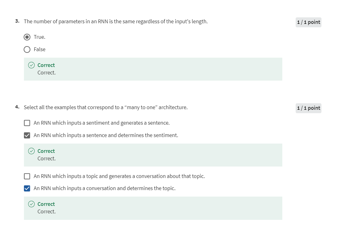
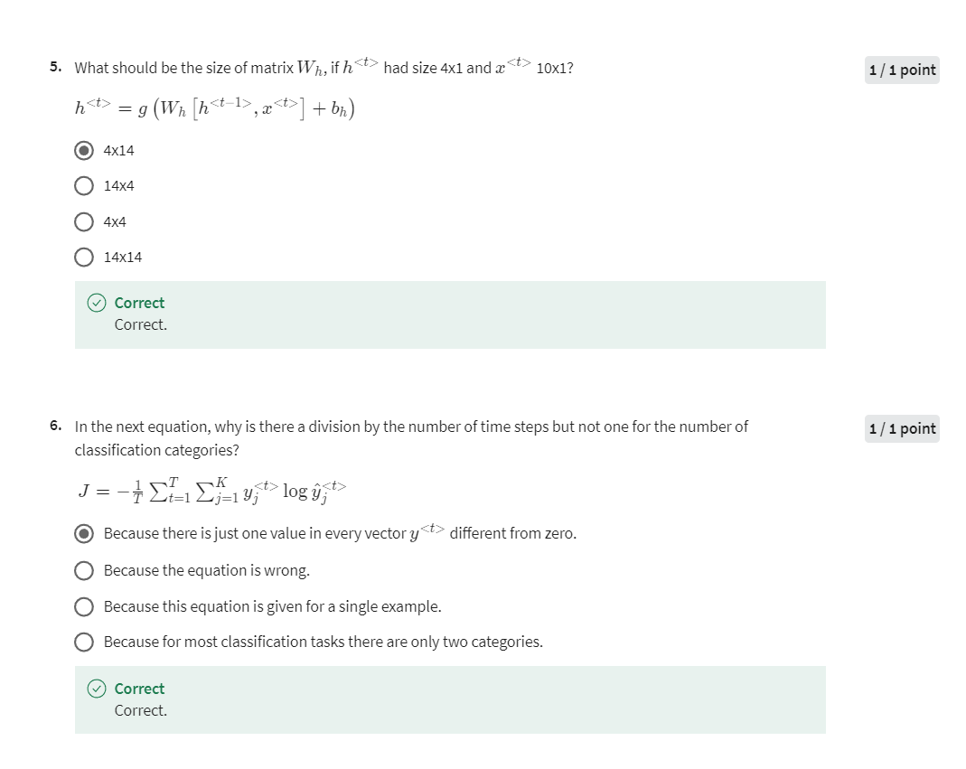
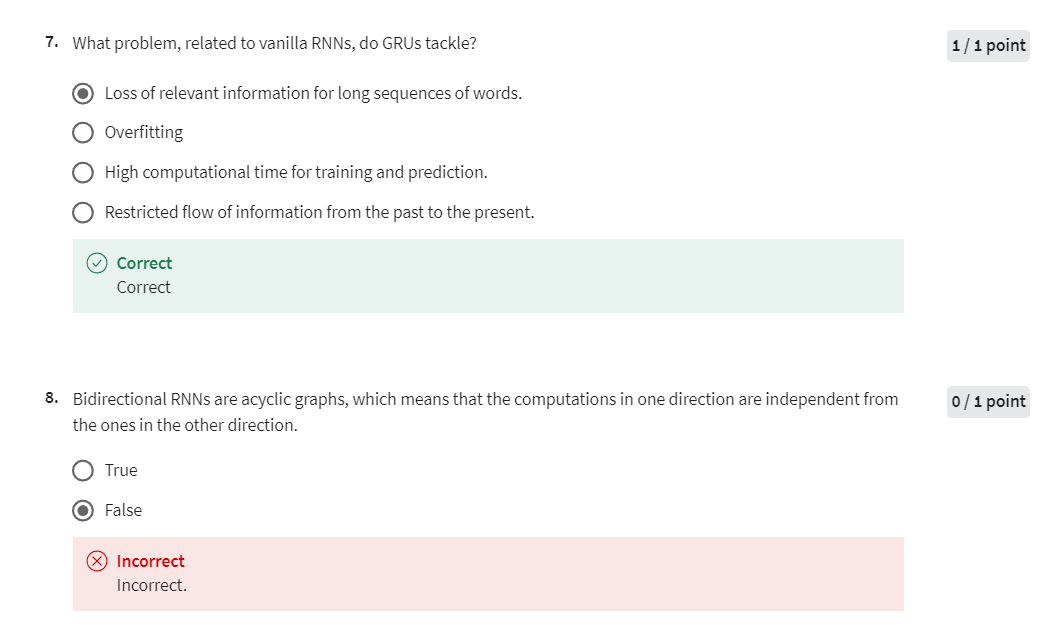
第八题改正:
双向 RNN 是无环图,这意味着一个方向的计算与另一个方向的计算无关。

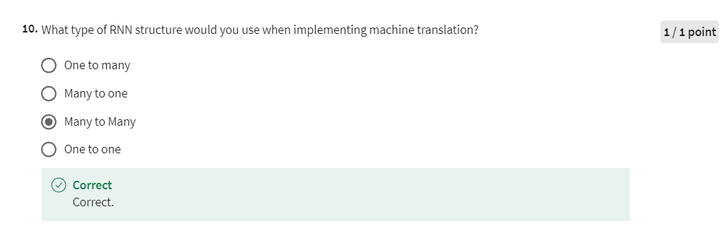
Programming Assignment: Deep N-grams
Assignment 1: Deep N-grams
Welcome to the first graded assignment of course 3. In this assignment you will explore Recurrent Neural Networks RNN.
In this notebook you will apply the following steps:
- Convert a line of text into a tensor
- Create a tensorflow dataset
- Define a GRU model using
TensorFlow - Train the model using
TensorFlow - Compute the accuracy of your model using the perplexity
- Generate text using your own model
Before getting started take some time to read the following tips:
TIPS FOR SUCCESSFUL GRADING OF YOUR ASSIGNMENT:
All cells are frozen except for the ones where you need to submit your solutions.
You can add new cells to experiment but these will be omitted by the grader, so don’t rely on newly created cells to host your solution code, use the provided places for this.
You can add the comment # grade-up-to-here in any graded cell to signal the grader that it must only evaluate up to that point. This is helpful if you want to check if you are on the right track even if you are not done with the whole assignment. Be sure to remember to delete the comment afterwards!
To submit your notebook, save it and then click on the blue submit button at the beginning of the page.
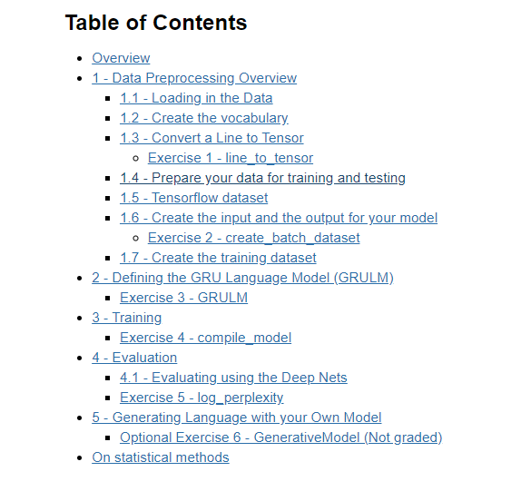
Overview
In this lab, you’ll delve into the world of text generation using Recurrent Neural Networks (RNNs). Your primary objective is to predict the next set of characters based on the preceding ones. This seemingly straightforward task holds immense practicality in applications like predictive text and creative writing.
The journey unfolds as follows:
Data Preprocessing: You’ll start by converting lines of text into numerical tensors, making them machine-readable.
Dataset Creation: Next, you’ll create a TensorFlow dataset, which will serve as the backbone for supplying data to your model.
Neural Network Training: Your model will be trained to predict the next set of characters, specifying the desired output length.
Character Embeddings: Character embeddings will be employed to represent each character as a vector, a fundamental technique in natural language processing.
GRU Model: Your model utilizes a Gated Recurrent Unit (GRU) to process character embeddings and make sequential predictions. The following figure gives you a summary of what you are about to implement.
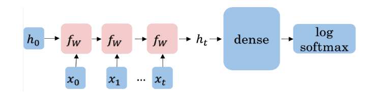
- Prediction Process: The model’s predictions are achieved through a linear layer and log-softmax computation.
This overview sets the stage for your exploration of text generation. Get ready to unravel the secrets of language and embark on a journey into the realm of creative writing and predictive text generation.
And as usual let’s start by importing all the required libraries.
import os
import traceback
os.environ['TF_CPP_MIN_LOG_LEVEL'] = '3'

import shutil
import numpy as np
import random as  rnd

import tensorflow as tf
from tensorflow.keras import layers
from tensorflow.keras.layers import Input

from termcolor import colored

# set random seed
rnd.seed(32)
import w1_unittest
1 - Data Preprocessing Overview

In this section, you will prepare the data for training your model. The data preparation involves the following steps:
Dataset Import: Begin by importing the dataset. Each sentence is structured as one line in the dataset. To ensure consistency, remove any extra spaces from these lines using the
stripfunction.Data Storage: Store each cleaned line in a list. This list will serve as the foundational dataset for your text generation task.
Character-Level Processing: Since the goal is character generation, it’s essential to process the text at the character level, not the word level. This involves converting each individual character into a numerical representation. To achieve this:
- Use the
tf.strings.unicode_splitfunction to split each sentence into its constituent characters. - Utilize
tf.keras.layers.StringLookupto map these characters to integer values. This transformation lays the foundation for character-based modeling.
- Use the
TensorFlow Dataset Creation: Create a TensorFlow dataset capable of producing data in batches. Each batch will consist of
batch_sizesentences, with each sentence containing a maximum ofmax_lengthcharacters. This organized dataset is essential for training your character generation model.
These preprocessing steps ensure that your dataset is meticulously prepared for the character-based text generation task, allowing you to work seamlessly with the Shakespearean corpus data.
1.1 - Loading in the Data
dirname = 'data/'
filename = 'shakespeare_data.txt'
lines = [] # storing all the lines in a variable.

counter = 0

with open(os.path.join(dirname, filename)) as files:
    for line in files:
        # remove leading and trailing whitespace
        pure_line = line.strip()#.lower()

        # if pure_line is not the empty string,
        if pure_line:
            # append it to the list
            lines.append(pure_line)

n_lines = len(lines)
print(f"Number of lines: {n_lines}")
Output: Number of lines: 125097
Let’s examine a few lines from the corpus. Pay close attention to the structure and style employed by Shakespeare in this excerpt. Observe that character names are written in uppercase, and each line commences with a capital letter. Your task in this exercise is to construct a generative model capable of emulating this particular structural style.
print("\n".join(lines[506:514]))
Output
BENVOLIO	Here were the servants of your adversary,
And yours, close fighting ere I did approach:
I drew to part them: in the instant came
The fiery Tybalt, with his sword prepared,
Which, as he breathed defiance to my ears,
He swung about his head and cut the winds,
Who nothing hurt withal hiss'd him in scorn:
While we were interchanging thrusts and blows,
1.2 - Create the vocabulary
In the following code cell, you will create the vocabulary for text processing. The vocabulary is a crucial component for understanding and processing text data. Here’s what the code does:
Concatenate all the lines in our dataset into a single continuous text, separated by line breaks.
Identify and collect the unique characters that make up the text. This forms the basis of our vocabulary.
To enhance the vocabulary, introduce two special characters:
- [UNK]: This character represents any unknown or unrecognized characters in the text.
- “” (empty character): This character is used for padding sequences when necessary.
The code concludes with the display of statistics, showing the total count of unique characters in the vocabulary and providing a visual representation of the complete character set.
text = "\n".join(lines)
# The unique characters in the file
vocab = sorted(set(text))
vocab.insert(0,"[UNK]") # Add a special character for any unknown
vocab.insert(1,"") # Add the empty character for padding.

print(f'{len(vocab)} unique characters')
print(" ".join(vocab))
Output
82 unique characters
[UNK]
   ! $ & ' ( ) , - . 0 1 2 3 4 5 6 7 8 9 : ; ? A B C D E F G H I J K L M N O P Q R S T U V W X Y Z [ ] a b c d e f g h i j k l m n o p q r s t u v w x y z |
1.3 - Convert a Line to Tensor
Now that you have your list of lines, you will convert each character in that list to a number using the order given by your vocabulary. You can use tf.strings.unicode_split to split the text into characters.
line = "Hello world!"
chars = tf.strings.unicode_split(line, input_encoding='UTF-8')
print(chars)
Output
tf.Tensor([b'H' b'e' b'l' b'l' b'o' b' ' b'w' b'o' b'r' b'l' b'd' b'!'], shape=(12,), dtype=string)
Using your vocabulary, you can convert the characters given by unicode_split into numbers. The number will be the index of the character in the given vocabulary.
print(vocab.index('a'))
print(vocab.index('e'))
print(vocab.index('i'))
print(vocab.index('o'))
print(vocab.index('u'))
print(vocab.index(' '))
print(vocab.index('2'))
print(vocab.index('3'))
Output
55
59
63
69
75
4
16
17
Tensorflow has a function tf.keras.layers.StringLookup that does this efficiently for list of characters. Note that the output object is of type tf.Tensor. Here is the result of applying the StringLookup function to the characters of “Hello world”
ids = tf.keras.layers.StringLookup(vocabulary=list(vocab), mask_token=None)(chars)
print(ids)
Output
tf.Tensor([34 59 66 66 69 4 77 69 72 66 58 5], shape=(12,), dtype=int64)
Exercise 1 - line_to_tensor
Instructions: Write a function that takes in a single line and transforms each character into its unicode integer. This returns a list of integers, which we’ll refer to as a tensor.
# GRADED FUNCTION: line_to_tensor
def line_to_tensor(line, vocab):
    """
    Converts a line of text into a tensor of integer values representing characters.

    Args:
        line (str): A single line of text.
        vocab (list): A list containing the vocabulary of unique characters.

    Returns:
        tf.Tensor(dtype=int64): A tensor containing integers (unicode values) corresponding to the characters in the `line`.
    """
    ### START CODE HERE ###

    # Split the input line into individual characters
    chars = tf.strings.unicode_split(line, input_encoding='UTF-8')
    # Map characters to their respective integer values using StringLookup
    ids = tf.keras.layers.StringLookup(vocabulary=list(vocab), mask_token=None)(chars)

    ### END CODE HERE ###

    return ids
# Test your function
tmp_ids = line_to_tensor('abc xyz', vocab)
print(f"Result: {tmp_ids}")
print(f"Output type: {type(tmp_ids)}")
Output
Result: [55 56 57  4 78 79 80]
Output type: <class 'tensorflow.python.framework.ops.EagerTensor'>
Expected output
Result: [55 56 57  4 78 79 80]
Output type: <class 'tensorflow.python.framework.ops.EagerTensor'>
# UNIT TEST
w1_unittest.test_line_to_tensor(line_to_tensor)
Output: All test passed!
You will also need a function that produces text given a numeric tensor. This function will be useful for inspection when you use your model to generate new text, because you will be able to see words rather than lists of numbers. The function will use the inverse Lookup function tf.keras.layers.StringLookup with invert=True in its parameters.
def text_from_ids(ids, vocab):
    """
    Converts a tensor of integer values into human-readable text.

    Args:
        ids (tf.Tensor): A tensor containing integer values (unicode IDs).
        vocab (list): A list containing the vocabulary of unique characters.

    Returns:
        str: A string containing the characters in human-readable format.
    """
    # Initialize the StringLookup layer to map integer IDs back to characters
    chars_from_ids = tf.keras.layers.StringLookup(vocabulary=vocab, invert=True, mask_token=None)

    # Use the layer to decode the tensor of IDs into human-readable text
    return tf.strings.reduce_join(chars_from_ids(ids), axis=-1)
Use the function for decoding the tensor produced by “Hello world!”
text_from_ids(ids, vocab).numpy()
Output
b'Hello world!'
1.4 - Prepare your data for training and testing
As usual, you will need some data for training your model, and some data for testing its performance. So, we will use 124097 lines for training and 1000 lines for testing.
train_lines = lines[:-1000] # Leave the rest for training
eval_lines = lines[-1000:] # Create a holdout validation set

print(f"Number of training lines: {len(train_lines)}")
print(f"Number of validation lines: {len(eval_lines)}")
Output
Number of training lines: 124097
Number of validation lines: 1000
1.5 - TensorFlow dataset
Most of the time in Natural Language Processing, and AI in general you use batches when training your models. Here, you will build a dataset that takes in some text and returns a batch of text fragments (Not necesarly full sentences) that you will use for training.
- The generator will produce text fragments encoded as numeric tensors of a desired length
Once you create the dataset, you can iterate on it like this:
data_generator.take(1)
This generator returns the data in a format that you could directly use in your model when computing the feed-forward of your algorithm. This batch dataset generator returns batches of data in an endless way.
So, let’s check how the different parts work with a corpus composed of 2 lines. Then, you will use these parts to create the first graded function of this notebook.
In order to get a dataset generator that produces batches of fragments from the corpus, you first need to convert the whole text into a single line, and then transform it into a single big tensor. This is only possible if your data fits completely into memory, but that is the case here.
all_ids = line_to_tensor("\n".join(["Hello world!", "Generative AI"]), vocab)
all_ids
Output
<tf.Tensor: shape=(26,), dtype=int64, numpy=
array([34, 59, 66, 66, 69,  4, 77, 69, 72, 66, 58,  5,  3, 33, 59, 68, 59,
       72, 55, 74, 63, 76, 59,  4, 27, 35])>
Create a dataset out of a tensor like input. This initial dataset will dispatch numbers in packages of a specified length. For example, you can use it for getting the 10 first encoded characters of your dataset. To make it easier to read, we can use the text_from_ids function.
ids_dataset = tf.data.Dataset.from_tensor_slices(all_ids)
print([text_from_ids([ids], vocab).numpy() for ids in ids_dataset.take(10)])
Output
[b'H', b'e', b'l', b'l', b'o', b' ', b'w', b'o', b'r', b'l']
But we can configure this dataset to produce batches of the same size each time. We could use this functionality to produce text fragments of a desired size (seq_length + 1). We will explain later why you need an extra character into the sequence.
seq_length = 10
data_generator = ids_dataset.batch(seq_length + 1, drop_remainder=True)
You can verify that the data generator produces encoded fragments of text of the desired length. For example, let’s ask the generator to produce 2 batches of data using the function data_generator.take(2)
for seq in data_generator.take(2):
    print(seq)
Output
tf.Tensor([34 59 66 66 69  4 77 69 72 66 58], shape=(11,), dtype=int64)
tf.Tensor([ 5  3 33 59 68 59 72 55 74 63 76], shape=(11,), dtype=int64)
But as usual, it is easier to understand if you print it in human readable characters using the ‘text_from_ids’ function.
i = 1
for seq in data_generator.take(2):
    print(f"{i}. {text_from_ids(seq, vocab).numpy()}")
    i = i + 1
Output
1. b'Hello world'
2. b'!\nGenerativ'
1.6 - Create the input and the output for your model
In this task you have to predict the next character in a sequence. The following function creates 2 tensors, each with a length of seq_length out of the input sequence of lenght seq_length + 1. The first one contains the first seq_length elements and the second one contains the last seq_length elements. For example, if you split the sequence ['H', 'e', 'l', 'l', 'o'], you will obtain the sequences ['H', 'e', 'l', 'l'] and ['e', 'l', 'l', 'o'].
def split_input_target(sequence):
    """
    Splits the input sequence into two sequences, where one is shifted by one position.

    Args:
        sequence (tf.Tensor or list): A list of characters or a tensor.

    Returns:
        tf.Tensor, tf.Tensor: Two tensors representing the input and output sequences for the model.
    """
    # Create the input sequence by excluding the last character
    input_text = sequence[:-1]
    # Create the target sequence by excluding the first character
    target_text = sequence[1:]

    return input_text, target_text
Look the result using the following sequence of characters
split_input_target(list("Tensorflow"))
Output
(['T', 'e', 'n', 's', 'o', 'r', 'f', 'l', 'o'],
 ['e', 'n', 's', 'o', 'r', 'f', 'l', 'o', 'w'])
The first sequence will be the input and the second sequence will be the expected output
Now, put all this together into a function to create your batch dataset generator
Exercise 2 - create_batch_dataset
Instructions: Create a batch dataset from the input text. Here are some things you will need.
- Join all the input lines into a single string. When you have a big dataset, you would better use a flow from directory or any other kind of generator.
- Transform your input text into numeric tensors
- Create a TensorFlow DataSet from your numeric tensors: Just feed the numeric tensors into the function
tf.data.Dataset.from_tensor_slices - Make the dataset produce batches of data that will form a single sample each time. This is, make the dataset produce a sequence of
seq_length + 1, rather than single numbers at each time. You can do it using thebatchfunction of the already created dataset. You must specify the length of the produced sequences (seq_length + 1). So, the sequence length produced by the dataset willseq_length + 1. It must have that extra element since you will get the input and the output sequences out of the same element.drop_remainder=Truewill drop the sequences that do not have the required length. This could happen each time that the dataset reaches the end of the input sequence. - Use the
split_input_targetto split each element produced by the dataset into the mentioned input and output sequences.The input will have the firstseq_lengthelements, and the output will have the lastseq_length. So, after this step, the dataset generator will produce batches of pairs (input, output) sequences. - Create the final dataset, using
dataset_xyas the starting point. You will configure this dataset to shuffle the data during the generation of the data with the specified BUFFER_SIZE. For performance reasons, you would like that tensorflow pre-process the data in parallel with training. That is calledprefetching, and it will be configured for you.
# GRADED FUNCTION: create_batch_dataset
def create_batch_dataset(lines, vocab, seq_length=100, batch_size=64):
    """
    Creates a batch dataset from a list of text lines.

    Args:
        lines (list): A list of strings with the input data, one line per row.
        vocab (list): A list containing the vocabulary.
        seq_length (int): The desired length of each sample.
        batch_size (int): The batch size.

    Returns:
        tf.data.Dataset: A batch dataset generator.
    """
    # Buffer size to shuffle the dataset
    # (TF data is designed to work with possibly infinite sequences,
    # so it doesn't attempt to shuffle the entire sequence in memory. Instead,
    # it maintains a buffer in which it shuffles elements).
    BUFFER_SIZE = 10000

    # For simplicity, just join all lines into a single line
    single_line_data  = "\n".join(lines)

    ### START CODE HERE ###

    # Convert your data into a tensor using the given vocab
    all_ids = line_to_tensor(single_line_data, vocab)
    # Create a TensorFlow dataset from the data tensor
    ids_dataset = tf.data.Dataset.from_tensor_slices(all_ids)
    # Create a batch dataset
    data_generator = ids_dataset.batch(seq_length + 1, drop_remainder=True)
    # Map each input sample using the split_input_target function
    dataset_xy = data_generator.map(split_input_target)

    # Assemble the final dataset with shuffling, batching, and prefetching
    dataset = (
        dataset_xy
        .shuffle(BUFFER_SIZE)
        .batch(batch_size, drop_remainder=True)
        .prefetch(tf.data.experimental.AUTOTUNE)
        )

    ### END CODE HERE ###

    return dataset
# test your function
tf.random.set_seed(1)
dataset = create_batch_dataset(train_lines[1:100], vocab, seq_length=16, batch_size=2)

print("Prints the elements into a single batch. The batch contains 2 elements: ")

for input_example, target_example in dataset.take(1):
    print("\n\033[94mInput0\t:", text_from_ids(input_example[0], vocab).numpy())
    print("\n\033[93mTarget0\t:", text_from_ids(target_example[0], vocab).numpy())

    print("\n\n\033[94mInput1\t:", text_from_ids(input_example[1], vocab).numpy())
    print("\n\033[93mTarget1\t:", text_from_ids(target_example[1], vocab).numpy())
Output
Prints the elements into a single batch. The batch contains 2 elements:

Input0	: b'and sight distra'

Target0	: b'nd sight distrac'


Input1	: b'when in his fair'

Target1	: b'hen in his fair '
Expected output
Prints the elements into a single batch. The batch contains 2 elements:

Input0	: b'and sight distra'

Target0	: b'nd sight distrac'


Input1	: b'when in his fair'

Target1	: b'hen in his fair '
# UNIT TEST
w1_unittest.test_create_batch_dataset(create_batch_dataset)
Output
All test passed!
1.7 - Create the training dataset
Now, you can generate your training dataset using the functions defined above. This will produce pairs of input/output tensors each time the batch generator creates an entry.
# Batch size
BATCH_SIZE = 64
dataset = create_batch_dataset(train_lines, vocab, seq_length=100, batch_size=BATCH_SIZE)
2 - Defining the GRU Language Model (GRULM)
Now that you have the input and output tensors, you will go ahead and initialize your model. You will be implementing the GRULM, gated recurrent unit model. To implement this model, you will be using TensorFlow. Instead of implementing the GRU from scratch (you saw this already in a lab), you will use the necessary methods from a built-in package. You can use the following packages when constructing the model:
tf.keras.layers.Embedding: Initializes the embedding. In this case it is the size of the vocabulary by the dimension of the model. docsEmbedding(vocab_size, embedding_dim).vocab_sizeis the number of unique words in the given vocabulary.embedding_dimis the number of elements in the word embedding (some choices for a word embedding size range from 150 to 300, for example).
tf.keras.layers.GRU:TensorFlowGRU layer. docs) Builds a traditional GRU of rnn_units with dense internal transformations. You can read the paper here: https://arxiv.org/abs/1412.3555units: Number of recurrent units in the layer. It must be set tornn_unitsreturn_sequences: It specifies if the model returns a sequence of predictions. Set it toTruereturn_state: It specifies if the model must return the last internal state along with the prediction. Set it toTrue
tf.keras.layers.Dense: A dense layer. docs. You must set the following parameters:units: Number of units in the layer. It must be set tovocab_sizeactivation: It must be set tolog_softmaxfunction as described in the next line.
tf.nn.log_softmax: Log of the output probabilities. docs- You don’t need to set any parameters, just set the activation parameter as
activation=tf.nn.log_softmax.
- You don’t need to set any parameters, just set the activation parameter as
Exercise 3 - GRULM
Instructions: Implement the GRULM class below. You should be using all the methods explained above.
# GRADED CLASS: GRULM
class GRULM(tf.keras.Model):
    """
    A GRU-based language model that maps from a tensor of tokens to activations over a vocabulary.

    Args:
        vocab_size (int, optional): Size of the vocabulary. Defaults to 256.
        embedding_dim (int, optional): Depth of embedding. Defaults to 256.
        rnn_units (int, optional): Number of units in the GRU cell. Defaults to 128.

    Returns:
        tf.keras.Model: A GRULM language model.
    """
    def __init__(self, vocab_size=256, embedding_dim=256, rnn_units=128):
        super().__init__(self)

        ### START CODE HERE ###

        # Create an embedding layer to map token indices to embedding vectors
        self.embedding = tf.keras.layers.Embedding(vocab_size, embedding_dim)
        # Define a GRU (Gated Recurrent Unit) layer for sequence modeling
        self.gru = tf.keras.layers.GRU(rnn_units, return_sequences=True, return_state=True)
        # Apply a dense layer with log-softmax activation to predict next tokens
        self.dense = tf.keras.layers.Dense(vocab_size, activation=tf.nn.log_softmax)

        ### END CODE HERE ###

    def call(self, inputs, states=None, return_state=False, training=False):
        x = inputs
        # Map input tokens to embedding vectors
        x = self.embedding(x, training=training)
        if states is None:
            # Get initial state from the GRU layer
            states = self.gru.get_initial_state(x)
        x, states = self.gru(x, initial_state=states, training=training)
        # Predict the next tokens and apply log-softmax activation
        x = self.dense(x, training=training)
        if return_state:
            return x, states
        else:
            return x
Now, you can define a new GRULM model. You must set the vocab_size to 82; the size of the embedding embedding_dim to 256, and the number of units that will have you recurrent neural network rnn_units to 512
# Length of the vocabulary in StringLookup Layer
vocab_size = 82

# The embedding dimension
embedding_dim = 256

# RNN layers
rnn_units = 512

model = GRULM(
    vocab_size=vocab_size,
    embedding_dim=embedding_dim,
    rnn_units = rnn_units)
# testing your model

try:
    # Simulate inputs of length 100. This allows to compute the shape of all inputs and outputs of our network
    model.build(input_shape=(BATCH_SIZE, 100))
    model.call(Input(shape=(100)))
    model.summary()
except:
    print("\033[91mError! \033[0mA problem occurred while building your model. This error can occur due to wrong initialization of the return_sequences parameter\n\n")
    traceback.print_exc()
Output
Model: "grulm"
_________________________________________________________________
 Layer (type)                Output Shape              Param #
=================================================================
 embedding (Embedding)       (None, 100, 256)          20992

 gru (GRU)                   [(None, 100, 512),        1182720
                              (None, 512)]

 dense (Dense)               (None, 100, 82)           42066

=================================================================
Total params: 1245778 (4.75 MB)
Trainable params: 1245778 (4.75 MB)
Non-trainable params: 0 (0.00 Byte)
_________________________________________________________________
Expected output
Model: "grulm"
_________________________________________________________________
 Layer (type)                Output Shape              Param #
=================================================================
 embedding (Embedding)    (None, 100, 256)          20992

 gru (GRU)                [(None, 100, 512),        1182720
                              (None, 512)]

 dense (Dense)            (None, 100, 82)           42066

=================================================================
Total params: 1245778 (4.75 MB)
Trainable params: 1245778 (4.75 MB)
Non-trainable params: 0 (0.00 Byte)
_________________________________________________________________
# UNIT TEST
w1_unittest.test_GRULM(GRULM)
Output
Test case 1:
All tests passed!
Test case 2:
All tests passed!
Now, let’s use the model for predicting the next character using the untrained model. At the begining the model will generate only gibberish.
for input_example_batch, target_example_batch in dataset.take(1):
    print("Input: ", input_example_batch[0].numpy()) # Lets use only the first sequence on the batch
    example_batch_predictions = model(tf.constant([input_example_batch[0].numpy()]))
    print("\n",example_batch_predictions.shape, "# (batch_size, sequence_length, vocab_size)")
Output
Input:  [73 62 55 66 74  4 62 69 66 58  4 74 62 59  4 69 70 63 68 63 69 68  4 69
 60  4 42 79 74 62 55 61 69 72 55 73  4 59 72 59  4 35  4 77 63 66 66  3
 55 66 66 69 77  4 69 60  4 74 62 79  4 77 63 74 73 11  4 55 68 58  4 60
 59 55 72  4 74 69  4 65 63 66 66  4 55  4 77 69 69 58 57 69 57 65 11  4
 66 59 73 74]

 (1, 100, 82) # (batch_size, sequence_length, vocab_size)
The output size is (1, 100, 82). We predicted only on the first sequence generated by the batch generator. 100 is the number of predicted characters. It has exactly the same length as the input. And there are 82 values for each predicted character. Each of these 82 real values are related to the logarithm likelihood of each character to be the next one in the sequence. The bigger the value, the higher the likelihood. As the network is not trained yet, all those values must be very similar and random. Just check the values for the last prediction on the sequence.
example_batch_predictions[0][99].numpy()
Output
array([-4.394292 , -4.40476  , -4.412511 , -4.3860574, -4.4002004,
       -4.406017 , -4.391721 , -4.412148 , -4.398938 , -4.409028 ,
       -4.4036393, -4.4032044, -4.412924 , -4.4294558, -4.4058275,
       -4.42735  , -4.4058037, -4.3803573, -4.400791 , -4.400802 ,
       -4.406753 , -4.3941684, -4.3932967, -4.4120283, -4.387955 ,
       -4.401387 , -4.409998 , -4.3959923, -4.3911653, -4.3927126,
       -4.418993 , -4.3965154, -4.4084926, -4.411369 , -4.3952107,
       -4.4010906, -4.3987713, -4.438392 , -4.395659 , -4.382313 ,
       -4.41321  , -4.3956714, -4.407373 , -4.4170127, -4.4092526,
       -4.3940024, -4.412472 , -4.4142866, -4.4282956, -4.4088607,
       -4.4279985, -4.412727 , -4.4195285, -4.4102244, -4.3989367,
       -4.4095216, -4.4144945, -4.3992176, -4.413693 , -4.400564 ,
       -4.4158244, -4.428811 , -4.41504  , -4.419681 , -4.416288 ,
       -4.4038076, -4.423907 , -4.413642 , -4.394232 , -4.419655 ,
       -4.4194393, -4.425377 , -4.40321  , -4.3787003, -4.411811 ,
       -4.386497 , -4.405401 , -4.3831735, -4.40585  , -4.428001 ,
       -4.410224 , -4.4233975], dtype=float32)
And the simplest way to choose the next character is by getting the index of the element with the highest likelihood. So, for instance, the prediction for the last characeter would be:
last_character = tf.math.argmax(example_batch_predictions[0][99])
print(last_character.numpy())
Output: 73
And the prediction for the whole sequence would be:
sampled_indices = tf.math.argmax(example_batch_predictions[0], axis=1)
print(sampled_indices.numpy())
Output
[21 27 71 12 73 41  6 75 75 48 72 77  6  6 41 75  4  3 28 28  3 14 18 75
 65 41 29 29 73  6 71  6 14 14 23 36 41 41 73 44 41 73 41 41 22 75  8 28
 25 12 12 75  5 41 75 74 41 29  6  6 41 41 22 77  3 17 54 41 50 48 41 29
 65 41 73 41 73 75 54  5  1 75  8 12 41 41 41 75 75 48 29 14 45  5 54 54
 12 70 21 73]
Those 100 numbers represent 100 predicted characters. However, humans cannot read this. So, let’s print the input and output sequences using our text_from_ids function, to check what is going on.
print("Input:\n", text_from_ids(input_example_batch[0], vocab))
print()
print("Next Char Predictions:\n", text_from_ids(sampled_indices, vocab))
Output
Input:
 tf.Tensor(b'shalt hold the opinion of Pythagoras ere I will\nallow of thy wits, and fear to kill a woodcock, lest', shape=(), dtype=string)

Next Char Predictions:
 tf.Tensor(b"7Aq-sO$uuVrw$$Ou \nBB\n04ukOCCs$q$009JOOsROsOO8u'B;--u!OutOC$$OO8w\n3]OXVOCkOsOsu]!u'-OOOuuVC0S!]]-p7s", shape=(), dtype=string)
As expected, the untrained model just produces random text as response of the given input. It is also important to note that getting the index of the maximum score is not always the best choice. In the last part of the notebook you will see another way to do it.
3 - Training
Now you are going to train your model. As usual, you have to define the cost function and the optimizer. You will use the following built-in functions provided by TensorFlow:
tf.losses.SparseCategoricalCrossentropy(): The Sparce Categorical Cross Entropy loss. It is the loss function used for multiclass classification.from_logits=True: This parameter informs the loss function that the output values generated by the model are not normalized like a probability distribution. This is our case, since our GRULM model uses alog_softmaxactivation rather than thesoftmax.
tf.keras.optimizers.Adam: Use Adaptive Moment Estimation, a stochastic gradient descent method optimizer that works well in most of the cases. Set thelearning_rateto 0.00125.
Exercise 4 - compile_model
Instructions: Compile the GRULM model using a SparseCategoricalCrossentropy loss and the Adam optimizer
# GRADED FUNCTION: Compile model
def compile_model(model):
    """
    Sets the loss and optimizer for the given model

    Args:
        model (tf.keras.Model): The model to compile.

    Returns:
        tf.keras.Model: The compiled model.
    """
    ### START CODE HERE ###

    # Define the loss function. Use SparseCategoricalCrossentropy
    loss = tf.losses.SparseCategoricalCrossentropy(from_logits=True)
    # Define and Adam optimizer
    opt = tf.keras.optimizers.Adam(learning_rate=0.00125)
    # Compile the model using the parametrized Adam optimizer and the SparseCategoricalCrossentropy funcion
    model.compile(optimizer=opt, loss=loss)

    ### END CODE HERE ###

    return model
## UNIT TEST
w1_unittest.test_compile_model(compile_model)
Output
All test passed!
Now, train your model for 10 epochs. With GPU this should take about one minute. With CPU this could take several minutes.
EPOCHS = 10

# Compile the model
model = compile_model(model)
# Fit the model
history = model.fit(dataset, epochs=EPOCHS)
Output
Epoch 1/10
790/790 [==============================] - 13s 12ms/step - loss: 2.0145
Epoch 2/10
790/790 [==============================] - 9s 10ms/step - loss: 1.4798
Epoch 3/10
790/790 [==============================] - 9s 10ms/step - loss: 1.3790
Epoch 4/10
790/790 [==============================] - 9s 10ms/step - loss: 1.3326
Epoch 5/10
790/790 [==============================] - 9s 10ms/step - loss: 1.3032
Epoch 6/10
790/790 [==============================] - 9s 10ms/step - loss: 1.2819
Epoch 7/10
790/790 [==============================] - 9s 10ms/step - loss: 1.2656
Epoch 8/10
790/790 [==============================] - 9s 10ms/step - loss: 1.2518
Epoch 9/10
790/790 [==============================] - 9s 10ms/step - loss: 1.2406
Epoch 10/10
790/790 [==============================] - 9s 10ms/step - loss: 1.2310
You can uncomment the following cell to save the weigthts of your model. This allows you to use the model later.
# # If you want, you can save the final model. Here is deactivated.
# output_dir = './your-model/'

# try:
#     shutil.rmtree(output_dir)
# except OSError as e:
#     pass

# model.save_weights(output_dir)
The model was only trained for 10 epochs. We pretrained a model for 30 epochs, which can take about 5 minutes in a GPU.
4 - Evaluation
4.1 - Evaluating using the Deep Nets
Now that you have learned how to train a model, you will learn how to evaluate it. To evaluate language models, we usually use perplexity which is a measure of how well a probability model predicts a sample. Note that perplexity is defined as:
P ( W ) = ∏ i = 1 N 1 P ( w i ∣ w 1 , . . . , w n − 1 ) N P(W) = \sqrt[N]{\prod_{i=1}^{N} \frac{1}{P(w_i| w_1,...,w_{n-1})}} P(W)=Ni=1∏NP(wi∣w1,...,wn−1)1
As an implementation hack, you would usually take the log of that formula (to enable us to use the log probabilities we get as output of our RNN, convert exponents to products, and products into sums which makes computations less complicated and computationally more efficient).
log P ( W ) = log ( ∏ i = 1 N 1 P ( w i ∣ w 1 , . . . , w n − 1 ) N ) \log P(W) = {\log\left(\sqrt[N]{\prod_{i=1}^{N} \frac{1}{P(w_i| w_1,...,w_{n-1})}}\right)} logP(W)=log
Ni=1∏NP(wi∣w1,...,wn−1)1
= log ( ( ∏ i = 1 N 1 P ( w i ∣ w 1 , . . . , w n − 1 ) ) 1 N ) = \log\left(\left(\prod_{i=1}^{N} \frac{1}{P(w_i| w_1,...,w_{n-1})}\right)^{\frac{1}{N}}\right) =log
(i=1∏NP(wi∣w1,...,wn−1)1)N1
= log ( ( ∏ i = 1 N P ( w i ∣ w 1 , . . . , w n − 1 ) ) − 1 N ) = \log\left(\left({\prod_{i=1}^{N}{P(w_i| w_1,...,w_{n-1})}}\right)^{-\frac{1}{N}}\right) =log
(i=1∏NP(wi∣w1,...,wn−1))−N1
= − 1 N log ( ∏ i = 1 N P ( w i ∣ w 1 , . . . , w n − 1 ) ) = -\frac{1}{N}{\log\left({\prod_{i=1}^{N}{P(w_i| w_1,...,w_{n-1})}}\right)} =−N1log(i=1∏NP(wi∣w1,...,wn−1)) = − 1 N ∑ i = 1 N log P ( w i ∣ w 1 , . . . , w n − 1 ) = -\frac{1}{N}{{\sum_{i=1}^{N}{\log P(w_i| w_1,...,w_{n-1})}}} =−N1i=1∑NlogP(wi∣w1,...,wn−1)
Exercise 5 - log_perplexity
Instructions: Write a program that will help evaluate your model. Implementation hack: your program takes in preds and target. preds is a tensor of log probabilities. You can use tf.one_hot to transform the target into the same dimension. You then multiply them and sum them. For the sake of simplicity, we suggest you use the NumPy functions sum, mean and equal, Good luck!
# GRADED FUNCTION: log_perplexity
def log_perplexity(preds, target):
    """
    Function to calculate the log perplexity of a model.

    Args:
        preds (tf.Tensor): Predictions of a list of batches of tensors corresponding to lines of text.
        target (tf.Tensor): Actual list of batches of tensors corresponding to lines of text.

    Returns:
        float: The log perplexity of the model.
    """
    PADDING_ID = 1
    ### START CODE HERE ###

    # Calculate log probabilities for predictions using one-hot encoding
    log_p = np.sum(preds * tf.one_hot(target, preds.shape[-1]), axis= -1) # HINT: tf.one_hot() should replace one of the Nones
    # Identify non-padding elements in the target
    non_pad = 1.0 - np.equal(target, PADDING_ID)          # You should check if the target equals to PADDING_ID
    # Apply non-padding mask to log probabilities to exclude padding
    log_p = log_p * non_pad                              # Get rid of the padding
    # Calculate the log perplexity by taking the sum of log probabilities and dividing by the sum of non-padding elements
    log_ppx = np.sum(log_p, axis=-1) / np.sum(non_pad, axis=-1) # Remember to set the axis properly when summing up
    # Compute the mean of log perplexity
    log_ppx = np.mean(log_ppx) # Compute the mean of the previous expression

    ### END CODE HERE ###
    return -log_ppx
#UNIT TESTS
w1_unittest.test_test_model(log_perplexity)
Output
All test passed!
Now load the provided pretrained model just to ensure that results are consistent for the upcoming parts of the notebook. You need to instantiate the GRULM model and then load the saved weights.
# Load the pretrained model. This step is optional.
vocab_size = len(vocab)
embedding_dim = 256
rnn_units = 512

model = GRULM(
    vocab_size=vocab_size,
    embedding_dim=embedding_dim,
    rnn_units = rnn_units)
model.build(input_shape=(100, vocab_size))
model.load_weights('./model/')
Now, you will use the 1000 lines of the corpus that were reserved at the begining of this notebook as test data. You will apply the same preprocessing as you did for the train dataset: get the numeric tensor from the input lines, and use the split_input_target to generate the inputs and the expected outputs.
Second, you will predict the next characters for the whole dataset, and you will compute the perplexity for the expected outputs and the given predictions.
#for line in eval_lines[1:3]:
eval_text = "\n".join(eval_lines)
eval_ids = line_to_tensor([eval_text], vocab)
input_ids, target_ids = split_input_target(tf.squeeze(eval_ids, axis=0))

preds, status = model(tf.expand_dims(input_ids, 0), training=False, states=None, return_state=True)

#Get the log perplexity
log_ppx = log_perplexity(preds, tf.expand_dims(target_ids, 0))
print(f'The log perplexity and perplexity of your model are {log_ppx} and {np.exp(log_ppx)} respectively')
Output
The log perplexity and perplexity of your model are 1.2239635591264044 and 3.400639693684683 respectively
Expected Output: The log perplexity and perplexity of your model are around 1.22 and 3.40 respectively.
So, the log perplexity of the model is 1.22. It is not an easy to interpret metric, but it can be used to compare among models. The smaller the value the better the model.
5 - Generating Language with your Own Model
Your GRULM model demonstrates an impressive ability to predict the most likely characters in a sequence, based on log scores. However, it’s important to acknowledge that this model, in its default form, is deterministic and can result in repetitive and monotonous outputs. For instance, it tends to provide the same answer to a question consistently.
To make your language model more dynamic and versatile, you can introduce an element of randomness into its predictions. This ensures that even if you feed the model in the same way each time, it will generate different sequences of text.
To achieve this desired behavior, you can employ a technique known as random sampling. When presented with an array of log scores for the N characters in your dictionary, you add an array of random numbers to this data. The extent of randomness introduced into the predictions is regulated by a parameter called “temperature”. By comparing the random numbers to the original input scores, the model adapts its choices, offering diversity in its outputs.
This doesn’t imply that the model produces entirely random results on each iteration. Rather, with each prediction, there is a probability associated with choosing a character other than the one with the highest score. This concept becomes more tangible when you explore the accompanying Python code.
def temperature_random_sampling(log_probs, temperature=1.0):
    """Temperature Random sampling from a categorical distribution. The higher the temperature, the more
       random the output. If temperature is close to 0, it means that the model will just return the index
       of the character with the highest input log_score

    Args:
        log_probs (tf.Tensor): The log scores for each characeter in the dictionary
        temperature (number): A value to weight the random noise.
    Returns:
        int: The index of the selected character
    """
   # Generate uniform random numbers with a slight offset to avoid log(0)
    u = tf.random.uniform(minval=1e-6, maxval=1.0 - 1e-6, shape=log_probs.shape)

    # Apply the Gumbel distribution transformation for randomness
    g = -tf.math.log(-tf.math.log(u))

    # Adjust the logits with the temperature and choose the character with the highest score
    return tf.math.argmax(log_probs + g * temperature, axis=-1)
Now, it’s time to bring all the elements together for the exciting task of generating new text. The GenerativeModel class plays a pivotal role in this process, offering two essential functions:
generate_one_step: This function is your go-to method for generating a single character at a time. It accepts two key inputs: an initial input sequence and a state that can be thought of as the ongoing context or memory of the model. The function delivers a single character prediction and an updated state, which can be used as the context for future predictions.generate_n_chars: This function takes text generation to the next level. It orchestrates the iterative generation of a sequence of characters. At each iteration, generate_one_step is called with the last generated character and the most recent state. This dynamic approach ensures that the generated text evolves organically, building upon the context and characters produced in previous steps. Each character generated in this process is collected and stored in the result list, forming the final output text.
Optional Exercise 6 - GenerativeModel (Not graded)
Instructions: Implementing the One-Step Generator
In this task, you will create a function to generate a single character based on the input text, using the provided vocabulary and the trained model. Follow these steps to complete the generate_one_step function:
Start by transforming your input text into a tensor using the given vocab. This will convert the text into a format that the model can understand.
Utilize the trained model with the input_ids and the provided states to predict the next characters. Make sure to retrieve the updated states from this prediction because they are essential for the final output.
Since we are only interested in the next character prediction, keep only the result for the last character in the sequence.
Employ the temperature random sampling technique to convert the vector of scores into a single character prediction. For this step, you will use the predicted_logits obtained in the previous step and the temperature parameter of the model.
To transform the numeric prediction into a human-readable character, use the text_from_ids function. Be mindful that text_from_ids expects a list as its input, so you need to wrap the output of the temperature_random_sampling function in square brackets […]. Don’t forget to use self.vocab as the second parameter for character mapping.
Finally, return the predicted_chars, which will be a single character, and the states tensor obtained from step 2. These components are essential for maintaining the sequence and generating subsequent characters.
# UNGRADED CLASS: GenerativeModel
class GenerativeModel(tf.keras.Model):
    def __init__(self, model, vocab, temperature=1.0):
        """
        A generative model for text generation.

        Args:
            model (tf.keras.Model): The underlying model for text generation.
            vocab (list): A list containing the vocabulary of unique characters.
            temperature (float, optional): A value to control the randomness of text generation. Defaults to 1.0.
        """
        super().__init__()
        self.temperature = temperature
        self.model = model
        self.vocab = vocab

    @tf.function
    def generate_one_step(self, inputs, states=None):
        """
        Generate a single character and update the model state.

        Args:
            inputs (string): The input string to start with.
            states (tf.Tensor): The state tensor.

        Returns:
            tf.Tensor, states: The predicted character and the current GRU state.
        """
        # Convert strings to token IDs.

        ### START CODE HERE ###

        # Transform the inputs into tensors
        input_ids = line_to_tensor(inputs, self.vocab)
        # Predict the sequence for the given input_ids. Use the states and return_state=True
        predicted_logits, states = self.model(input_ids, states=states, return_state=True)
        # Get only last element of the sequence
        predicted_logits = predicted_logits[0, -1, :]
        # Use the temperature_random_sampling to generate the next character.
        predicted_ids = temperature_random_sampling(predicted_logits, self.temperature)
        # Use the chars_from_ids to transform the code into the corresponding char
        predicted_chars = text_from_ids([predicted_ids], self.vocab)

        ### END CODE HERE ###

        # Return the characters and model state.
        return tf.expand_dims(predicted_chars, 0), states

    def generate_n_chars(self, num_chars, prefix):
        """
        Generate a text sequence of a specified length, starting with a given prefix.

        Args:
            num_chars (int): The length of the output sequence.
            prefix (string): The prefix of the sequence (also referred to as the seed).

        Returns:
            str: The generated text sequence.
        """
        states = None
        next_char = tf.constant([prefix])
        result = [next_char]
        for n in range(num_chars):
            next_char, states = self.generate_one_step(next_char, states=states)
            result.append(next_char)

        return tf.strings.join(result)[0].numpy().decode('utf-8')
# UNIT TEST
# Fix the seed to get replicable results for testing
tf.random.set_seed(272)
gen = GenerativeModel(model, vocab, temperature=0.5)

print(gen.generate_n_chars(32, " "), '\n\n' + '_'*80)
print(gen.generate_n_chars(32, "Dear"), '\n\n' + '_'*80)
print(gen.generate_n_chars(32, "KING"), '\n\n' + '_'*80)
Output
 hear he has a soldier.
Here is a

________________________________________________________________________________
Dear gold, if thou wilt endure the e

________________________________________________________________________________
KING OF THE SHREW
IV	I beseech you,

________________________________________________________________________________
Expected output
 hear he has a soldier.
Here is a

________________________________________________________________________________
Dear gold, if thou wilt endure the e

________________________________________________________________________________
KING OF THE SHREW
IV	I beseech you,

________________________________________________________________________________
w1_unittest.test_GenerativeModel(GenerativeModel, model, vocab)
Output
All test passed!
Now, generate a longer text. Let’s check if it looks like Shakespeare fragment
tf.random.set_seed(np.random.randint(1, 1000))
gen = GenerativeModel(model, vocab, temperature=0.8)
import time
start = time.time()
print(gen.generate_n_chars(1000, "ROMEO "), '\n\n' + '_'*80)
print('\nRun time:', time.time() - start)
Output
ROMEO and EDGAR]
YORK	O, holy them, Capilet in the sea,
Which is the blood of singularight
And makes the brothel of his side. You'll follow
The entreaty of your father lost,
And we for any upon's stained him for death,
I will survey me to the picture of fight,
To be thy necessity of this feast
with pox on the block of harlots.
CARDINAL	Who hears our general. Here, sir.
[Second Fisherman.
[Enter PERDITAlus, I will place the wrestler,
All the crown of Salicrous knave to set it
dires and feigning but that ring, the word,
Save that his offence in succession,
I tell thee, my most virtues of perfection of
the streets, to flatter him to thy father, be cauce on.
ERPINGHAM	No, let me fall down the resisting piece
In bloody gazers, or I shall think the nobles
Which in the water of eyes be advanced the fortune
From such weapons, the be a special of horse will make
Engages out o' the chaff as many galloars,
With your head again, out of the loss of all I
have a glove within my money.
QUEEN MARGARET	But,

________________________________________________________________________________

Run time: 2.659285545349121
In the generated text above, you can see that the model generates text that makes sense capturing dependencies between words and without any input. A simple n-gram model would have not been able to capture all of that in one sentence.
On statistical methods
Using a statistical method like the one you implemented in course 2 will not give you results that are as good as you saw here. Your model will not be able to encode information seen previously in the data set and as a result, the perplexity will increase. Remember from course 2 that the higher the perplexity, the worse your model is. Furthermore, statistical ngram models take up too much space and memory. As a result, they will be inefficient and too slow. Conversely, with deepnets, you can get a better perplexity. Note, learning about n-gram language models is still important and allows you to better understand deepnets.
Grades
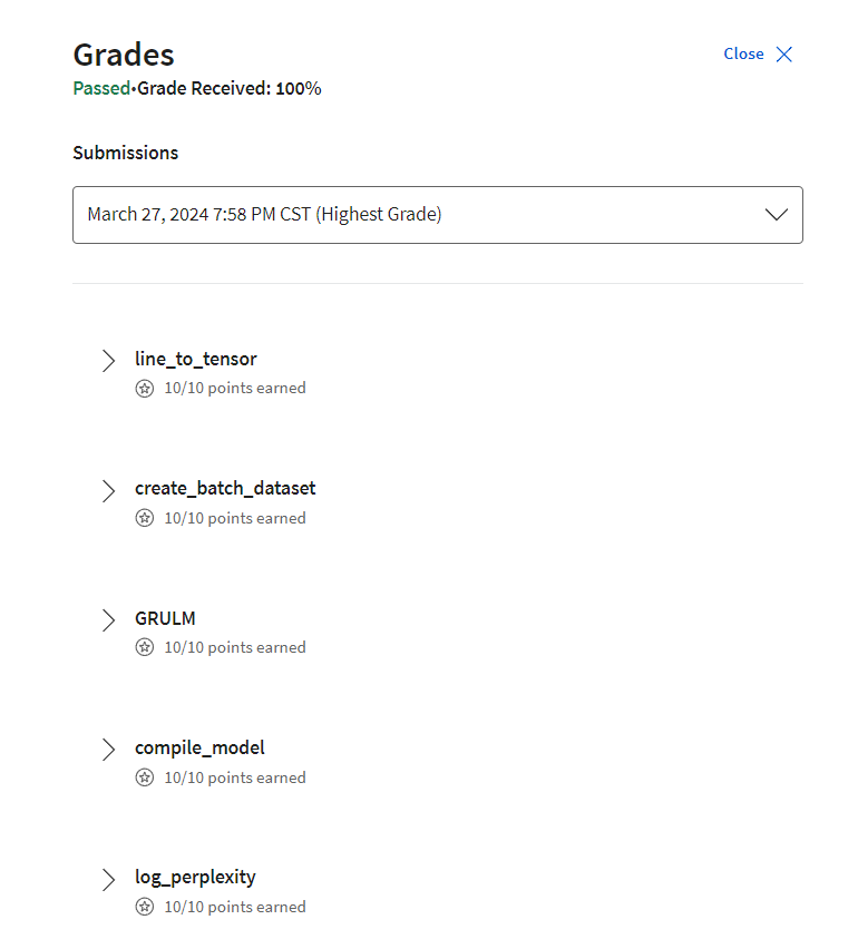
参考:https://www.kaggle.com/code/seshupavan/shakespeare-text-generation-using-tensorflow
后记
2024年3月27日早上开始学习Natural Language Processing with Sequence Models这门课,截至2024年3月27日20点00分,完成week 1的学习。这周对RNN和GRU的原理有了更深的了解,并且在TensorFlow框架下实现了某些功能。由于之前有过PyTorch框架使用GRU和RNN的经历,现在可以通过tf横向对比学习,对自己功力的提升有所裨益。