以Breast cancer wisconsin (diagnostic) dataset数据集为例。
# Built-in libraries
import math
import numpy    as np
import pandas   as pd


# Visualization libraries
import matplotlib.pyplot as plt
import seaborn           as sns


# Sklearn libraries
#
from sklearn                 import metrics
from sklearn                 import preprocessing
from sklearn.model_selection import train_test_split
from sklearn.datasets        import load_breast_cancer
Parameters
test_size = 0.1Breast cancer wisconsin (diagnostic) dataset
Data Set Characteristics:
:Number of Instances: 569

:Number of Attributes: 30 numeric, predictive attributes and the class

:Attribute Information:
    - radius (mean of distances from center to points on the perimeter)
    - texture (standard deviation of gray-scale values)
    - perimeter
    - area
    - smoothness (local variation in radius lengths)
    - compactness (perimeter^2 / area - 1.0)
    - concavity (severity of concave portions of the contour)
    - concave points (number of concave portions of the contour)
    - symmetry
    - fractal dimension ("coastline approximation" - 1)

    The mean, standard error, and "worst" or largest (mean of the three
    largest values) of these features were computed for each image,
    resulting in 30 features.  For instance, field 3 is Mean Radius, field
    13 is Radius SE, field 23 is Worst Radius.

    - class:
            - WDBC-Malignant
            - WDBC-Benign

:Summary Statistics:

:Missing Attribute Values: None

:Class Distribution: 212 - Malignant, 357 - Benign
# Load Breast Cancer dataset
data = load_breast_cancer()


# Create DataFrame
#
df   = pd.DataFrame(data.data, columns=data.feature_names)
# Add a target column
#
df['class'] = data.target


# Show DataFrame
df.head(3)
#Pre-processing data
fig = plt.figure(figsize=(8
,3
))ax  = sns.countplot(df['class'], order = df['class'].value_counts().index)


#Create annotate
for i in ax.patches:
    ax.text(x        = i.get_x() + i.get_width()/2,
            y        = i.get_height()/7,
            s        = f"{np.round(i.get_height()/len(df)*100)}%",
            ha       = 'center',
            size     = 15,
            weight   = 'bold',
            rotation = 90,
            color    = 'white');


plt.title("Class variable", size=12, weight='bold');
Training/Testing sets
X = df.iloc[:,:-1]
Y = df.iloc[:, -1]
trainX, testX, trainY, testY = train_test_split(X, Y, test_size=test_size, random_state=42)
Model development
Setup ML model
from sklearn.ensemble import GradientBoostingClassifier


# XGBoost model
#
model = GradientBoostingClassifier( random_state  = 42 )
Training ML model
model.fit(trainX, trainY);
model.fit(trainX, trainY);
Get Predictions
# Calculate prediction
#
pred = model.predict( testX )


# Performance accuracy
#
accuracy = metrics.accuracy_score(testY, pred)
print("Accuracy: %.2f%%" % (accuracy * 100.0))
Accuracy: 96.49%
SHAP
%%capture
! pip install shap
import shap
# Generate the Tree explainer and SHAP values
explainer = shap.TreeExplainer(model)
shap_values = explainer.shap_values(X)
expected_value = explainer.expected_valueExplainability/Visualizations
Summary dot plot
# Generate summary dot plot
#
shap.summary_plot(shap_values   = shap_values,
                  features      = X,
                  feature_names = df.columns[:-1],
                  title         = 'SHAP summary plot')
Summary bar plot
# Generate summary bar plot
#
shap.summary_plot(shap_values   = shap_values,
                  features      = X,
                  feature_names = df.columns[:-1],
                  plot_type     = "bar")
Dependence plot
# Generate dependence plot
#
shap.dependence_plot(ind               = "worst concave points",
                     shap_values       = shap_values,
                     features          = X,
                     feature_names     = df.columns[:-1],
                     interaction_index = "mean concave points")
Multiple dependence plots
# Generate multiple dependence plots
for name in df.columns[:-1]:
     shap.dependence_plot(ind               = name,
                          shap_values       = shap_values,
                          features          = X,
                          feature_names     = df.columns[:-1],)


工学博士,担任《Mechanical System and Signal Processing》《中国电机工程学报》《控制与决策》等期刊审稿专家,擅长领域:现代信号处理,机器学习,深度学习,数字孪生,时间序列分析,设备缺陷检测、设备异常检测、设备智能故障诊断与健康管理PHM等。

