Coursera吴恩达深度学习专项课程01: Neural Networks and Deep Learning 学习笔记 Week 04 （完结）

Neural Networks and Deep Learning

Course Certificate

本文是学习 https://www.coursera.org/learn/neural-networks-deep-learning 这门课的笔记

Course Intro

Week 04: Deep Neural Networks

Analyze the key computations underlying deep learning, then use them to build and train deep neural networks for computer vision tasks.

Learning Objectives

---

• Describe the successive block structure of a deep neural network
• Build a deep L-layer neural network
• Analyze matrix and vector dimensions to check neural network implementations
• Use a cache to pass information from forward to back propagation
• Explain the role of hyperparameters in deep learning
• Build a 2-layer neural network

Deep L-layer Neural Network

Welcome to the fourth week of this course. By now, you’ve seen forward propagation and
back propagation in the context of a neural network, with a single hidden
layer, as well as logistic regression, and you’ve learned about vectorization, and when it’s important to
initialize the ways randomly. If you’ve done the past couple weeks
homework, you’ve also implemented and seen some of these ideas work for
yourself. So by now, you’ve actually seen most of the ideas you
need to implement a deep neural network. What we’re going to do this week, is take
those ideas and put them together so that you’ll be able to implement
your own deep neural network. Because this week’s problem
exercise is longer, it just has been more work,
I’m going to keep the videos for this week shorter as you can get through
the videos a little bit more quickly, and then have more time to do a significant
problem exercise at then end, which I hope will leave you having thoughts deep in
neural network, that if you feel proud of.

shallow vs. deep NN

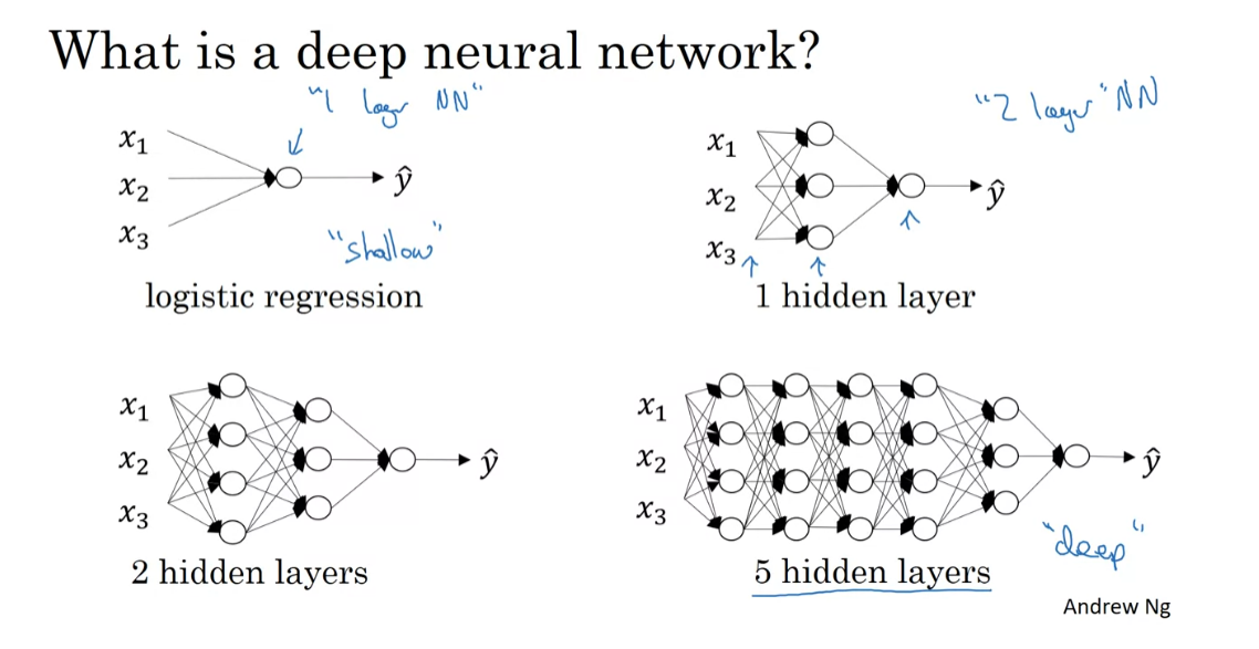
So what is a deep neural network? You’ve seen this picture for
logistic regression and you’ve also seen neural networks
with a single hidden layer. So here’s an example of a neural
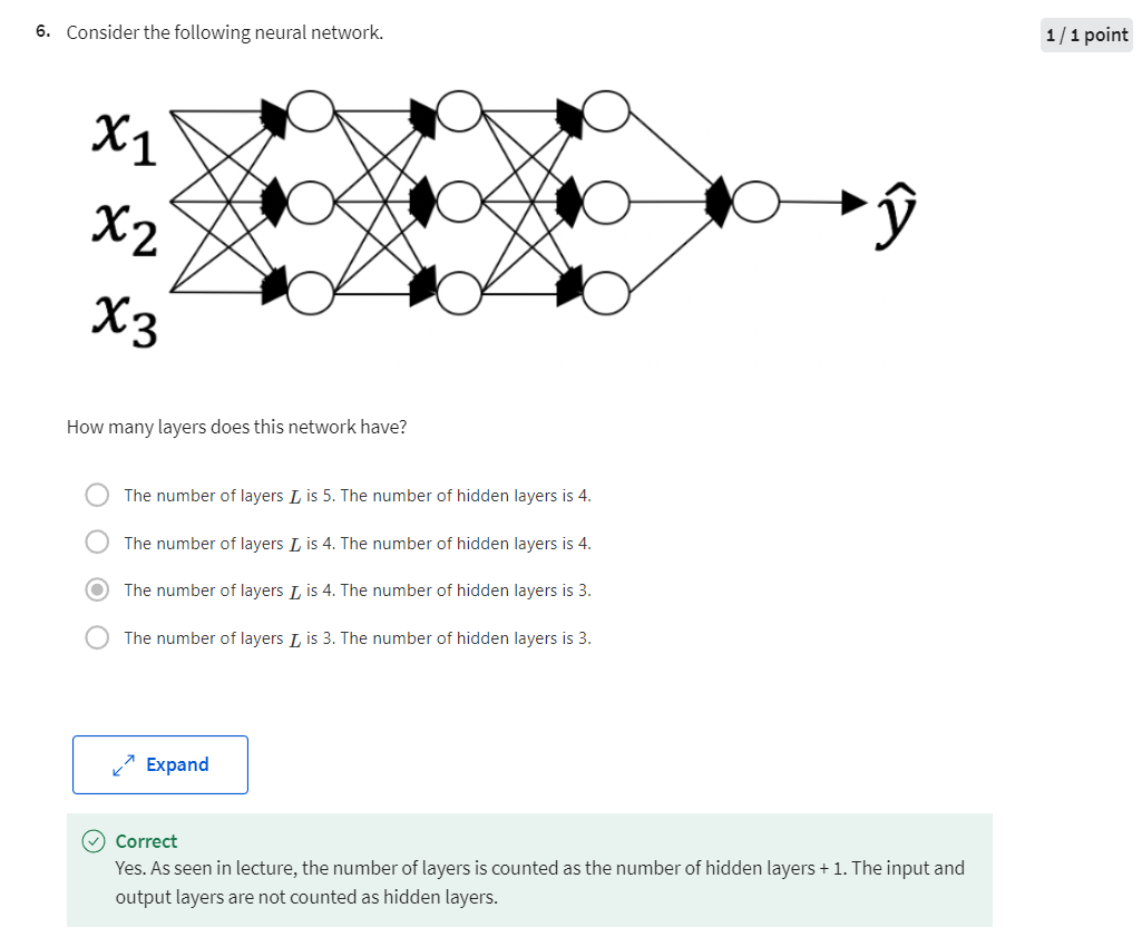
network with two hidden layers and a neural network with 5 hidden layers. We say that logistic regression
is a very “shallow” model, whereas this model here is
a much deeper model, and shallow versus depth
is a matter of degree. So neural network of
a single hidden layer, this would be a 2 layer neural network. Remember when we count layers in a neural
network, we don’t count the input layer, we just count the hidden layers
as was the output layer. So, this would be a 2 layer neural
network is still quite shallow, but not as shallow as logistic regression. Technically logistic regression
is a one layer neural network, we could then, but
over the last several years the AI, on the machine learning community,
has realized that there are functions that very deep neural networks can learn that
shallower models are often unable to. Although for any given problem, it might
be hard to predict in advance exactly how deep in your network you would want. So it would be reasonable to try
logistic regression, try one and then two hidden layers, and view the
number of hidden layers as another hyper parameter that you could try
a variety of values of, and evaluate on all that across validation
data, or on your development set. See more about that later as well.

notation of deep NN

Let’s now go through the notation we
used to describe deep neural networks. Here’s is a one, two, three,
four layer neural network, With three hidden layers, and
the number of units in these hidden layers are I guess 5, 5, 3, and
then there’s one one upper unit. So the notation we’re going to use, is going to use capital L ,to denote
the number of layers in the network. So in this case, L = 4, and so
does the number of layers, and we’re going to use N superscript
[l] to denote the number of nodes, or the number of units
in layer lowercase l. So if we index this,
the input as layer “0”. This is layer 1, this is layer 2,
this is layer 3, and this is layer 4. Then we have that, for example,
n[1], that would be this, the first is in there will equal 5,
because we have 5 hidden units there. For this one, we have the n[2], the number of units in
the second hidden layer is also equal to 5, n[3] = 3, and n[4] = n[L] this number
of upper units is 01, because your capital L is equal to four, and we’re also going to have here that for the input layer n[0] = nx = 3.

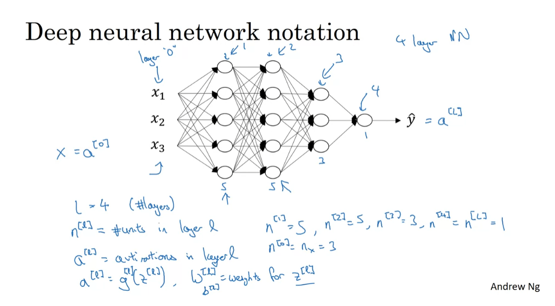
So that’s the notation we use to describe
the number of nodes we have in different layers. For each layer L, we’re also going to use a[l] to denote the activations in layer l. So we’ll see later that in for
propagation, you end up computing a[l] as
the activation g(z[l]) and perhaps the activation is
indexed by the layer l as well, and then we’ll use W[l ]to denote,
the weights for computing the value z[l] in layer l, and similarly, b[l] is used to compute z [l]. Finally, just to wrap up on the notation,
the input features are called x, but x is also the activations
of layer zero, so a[0] = x, and the activation of the final layer,
a[L] = y-hat. So a[L] is equal to the predicted output
to prediction y-hat to the neural network.

So you now know what a deep
neural network looks like, as was the notation we’ll use to describe
and to compute with deep networks. I know we’ve introduced a lot of notation
in this video, but if you ever forget what some symbol means, we’ve also posted
on the course website, a notation sheet or a notation guide, that you can use to look
up what these different symbols mean. Next, I’d like to describe what forward
propagation in this type of network looks like. Let’s go into the next video.

Forward Propagation in a Deep Network

see how you can perform forward propagation

In the last video, we described what is a deep L-layer neural network
and also talked about the notation we use to
describe such networks. In this video, you see how you can
perform forward propagation, in a deep network. As usual, let’s first go over what forward propagation will look like
for a single training example x, and then later on we’ll talk about
the vectorized version, where you want to carry out
forward propagation on the entire training set
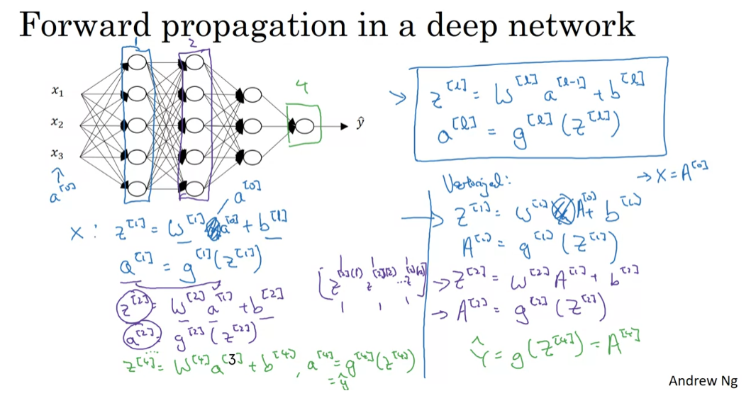
at the same time. But given a single training example x, here’s how you compute the
activations of the first layer. So for this first layer, you compute z1 equals w1 times x plus b1. So w1 and b1 are the parameters that
affect the activations in layer one. This is layer one of the neural network, and then you compute the activations
for that layer to be equal to g of z1. The activation function g
depends on what layer you’re at and maybe what index set as the
activation function from layer one. So if you do that, you’ve now computed
the activations for layer one. How about layer two? Say that layer. Well, you would then compute z2 equals w2 a1 plus b2. Then, so the activation of layer two is
the y matrix times the outputs of layer one. So, it’s that value, plus the bias vector for layer two. Then a2 equals the activation function
applied to z2. Okay? So that’s it for layer two, and so on and so forth. Until you get to the upper layer,
that’s layer four. Where you would have that z4 is equal to the parameters for that layer times
the activations from the previous layer, plus that bias vector. Then similarly, a4 equals g of z4. So, that’s how you compute your
estimated output, y hat. So, just one thing to notice, x here is also equal to a0, because the input feature vector x is
also the activations of layer zero. So we scratch out x. When I cross out x and put a0 here, then all of these equations
basically look the same.

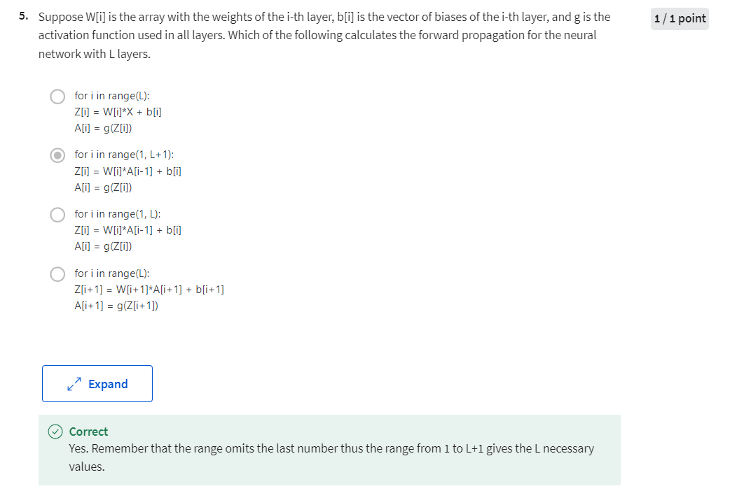
The general rule is that zl is equal to wl times a of l minus 1 plus bl. It’s one there. And then, the activations for that layer is the activation function
applied to the values of z. So, that’s the general
forward propagation equation. So, we’ve done all this for a
single training example.

vectorized version of forward propagation

How about for doing it in a vectorized way
for the whole training set at the same time? The equations look quite similar as before. For the first layer, you would
have capital Z1 equals w1 times capital X plus b1. Then, A1 equals g of Z1. Bear in mind that X is equal to A0. These are just the training examples
stacked in different columns. You could take this, let me scratch out X, they can put A0 there. Then for the next layer, looks similar, Z2 equals w2 A1 plus b2 and A2 equals g of Z2. We’re just taking these
vectors z or a and so on, and stacking them up. This is z vector for the
first training example, z vector for the
second training example, and so on, down to the
nth training example, stacking these and columns
and calling this capital Z. Similarly, for capital A, just as capital X. All the training examples are
column vectors stack left to right. In this process, you end up with
y hat which is equal to g of Z4, this is also equal to A4. That’s the predictions on all of your
training examples stacked horizontally.

So just to summarize on notation, I’m going to modify this up here. A notation allows us to replace lowercase z
and a with the uppercase counterparts, is that already looks like a capital Z. That gives you the vectorized version of forward propagation that you carry out
on the entire training set at a time, where A0 is X. Now, if you look at this
implementation of vectorization, it looks like that there is
going to be a For loop here. So therefore l equals 1-4. For L equals 1 through capital L. Then you
have to compute the activations for layer one, then layer two, then for layer three, and then the layer four. So, seems that there is a For loop here. I know that when implementing
neural networks, we usually want to get rid of
explicit For loops. But this is one place where I don’t think there’s any way to implement this
without an explicit For loop. So when implementing forward propagation, it is perfectly okay to have a For loop
to compute the activations for layer one, then layer two, then layer three,
then layer four. No one knows, and I don’t think
there is any way to do this without a For loop that
goes from one to capital L, from one through the total number of
layers in the neural network. So, in this place, it’s perfectly
okay to have an explicit For loop.

Next video

So, that’s it for the notation
for deep neural networks, as well as how to do forward propagation
in these networks. If the pieces we’ve seen so far
looks a little bit familiar to you, that’s because what we’re seeing is taking
a piece very similar to what you’ve seen in the neural network with a single hidden
layer and just repeating that more times. Now, it turns out that we implement
a deep neural network, one of the ways to increase your
odds of having a bug-free implementation is to think very systematic and carefully about the matrix
dimensions you’re working with. So, when I’m trying to debug my own code, I’ll often pull a piece of paper, and just think carefully through, so the dimensions of the
matrix I’m working with. Let’s see how you could
do that in the next video.

Getting your Matrix Dimensions Right

When implementing a
deep neural network, one of the debugging
tools I often use to check the
correctness of my code is to pull a piece
of paper and just work through the dimensions
in matrix I’m working with. Let me show you how to do
that since I hope this will make it easier for you to implement your deep
networks as well.

work through the dimensions in matrix

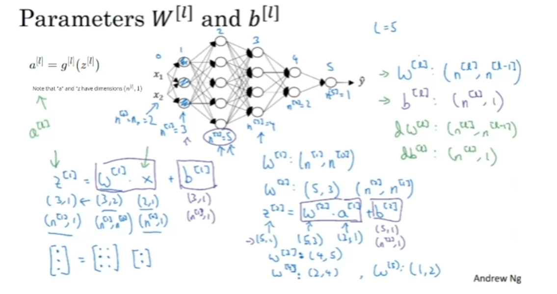
So capital L is equal to 5. I counted them quickly. Not counting the input layer, there are five layers here, four hidden layers
and one output layer. If you implement
forward propagation, the first step will be Z1 equals W1 times the input
features x plus b1. Let’s ignore the bias terms B for now and focus on
the parameters W. Now, this first hidden layer
has three hidden units. So this is Layer 0, Layer 1, Layer 2, Layer 3, Layer 4, and Layer 5. Using the notation we had
from the previous video, we have that n1, which is the number of hidden
units in layer 1, is equal to 3. Here we would have
that n2 is equal to 5, n3 is equal to 4, n4 is equal to 2, and n5 is equal to 1. So far we’ve only seen neural networks with
a single output unit, but in later courses
we’ll talk about neural networks with multiple
output units as well. Finally, for the input layer, we also have n0 equals
nX is equal to 2. Now, let’s think about the
dimensions of Z, W, and X. Z is the vector of activations for this first hidden layer. So Z is going to be 3 by 1, is going to be a
three-dimensional vector. I’m going to write it as, n1
by one-dimensional matrix, 3 by 1 in this case. Now, how about the
input features x? X we have two input features. So x is, in this example, 2 by 1, but more generally
it’ll be n0 by 1. What we need is for the
matrix W1 to be something that when we multiply an
n0 by 1 vector to it, we get an n1 by 1 vector. So you have a
three-dimensional vector equals something times a
two-dimensional vector. By the rules of matrix
multiplication, this has got to be
a 3 by 2 matrix. Because a 3 by 2
matrix times a 2 by 1 matrix or times
a 2 by 1 vector, that gives you a 3 by 1 vector. More generally,
this is going to be an n1 by n0 dimensional matrix.

So what we figured out here
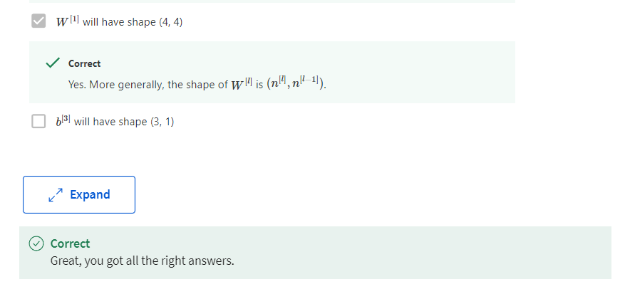
is that the dimensions of W1 has to be n1 by n0, and more generally,
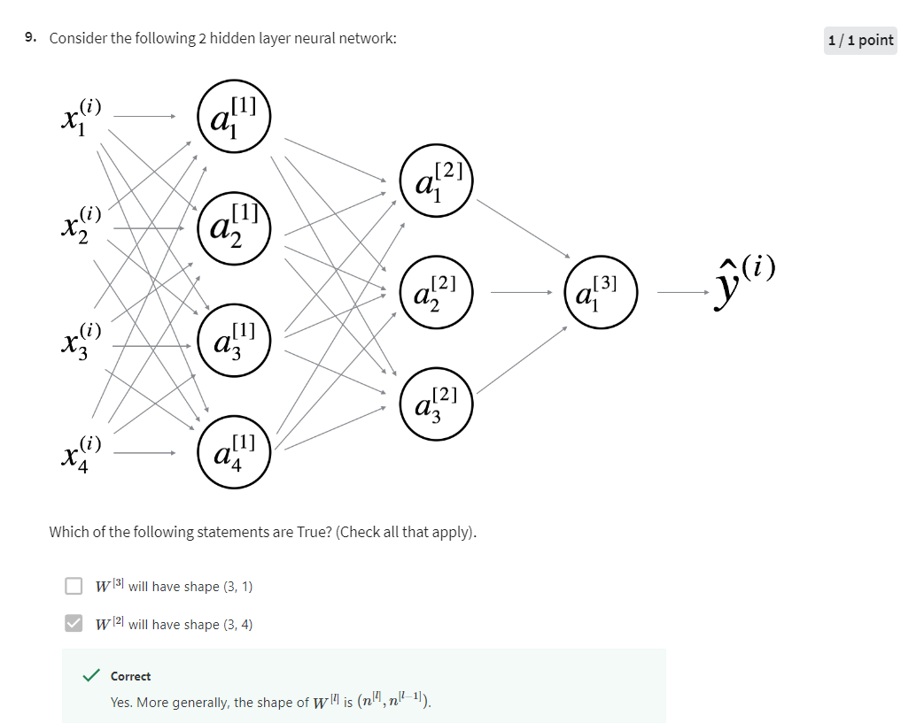
the dimensions of WL must be nL by nL minus 1. For example, the
dimensions of W2, for this, it will
have to be 5 by 3, or it will be n2 by n1, because we’re going
to compute Z2 as W2 times a1. Again, let’s ignore
the bias for now. This is going to be 3 by 1. We need this to be 5 by 1. So this had better be 5 by 3. Similarly, W3 is really the
dimension of the next layer, the dimension of
the previous layer. So this is going to be 4 by 5. W4 is going to be 2 by 4, and W5 is going to be 1 by 2. The general formula to
check is that when you’re implementing the
matrix for a layer L, that the dimension of that
matrix be nL by nL minus 1.

dimension of vector b

Now, let’s think about the
dimension of this vector B. This is going to be
a 3 by 1 vector, so you have to add
that to another 3 by 1 vector in order to get a 3
by 1 vector as the output. This was going to be 5 by 1, so there’s going to be
another 5 by 1 vector in order for the sum of these two things that
I have in the boxes to be itself a 5 by 1 vector. The more general rule is that
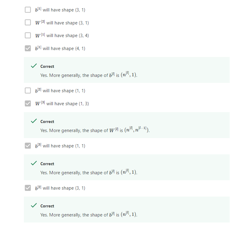
in the example on the left, b^ [1] is n^ [1] by 1, like this 3 by 1. In the second example, it is this is n^ [2] by 1 and so the more general
case is that b^ [l] should be n^ [l]
by 1 dimensional. Hopefully, these two
equations help you to double-check that the
dimensions of your matrices, w, as well as of your vectors b are the
correct dimensions.

Of course, if you’re
implementing back-propagation, then the dimensions of dw should be the
same as dimension of w. So dw should be the
same dimension as w, and db should be the
same dimension as b. Now, the other key
set of quantities whose dimensions to
check are these z, x, as well as a of l, which we didn’t talk
too much about here. But because z of l is
equal to g of a of l, apply element-wise then z and a should have the same dimension in these types of networks.

vectorized implementation and its dimension

Now, let’s see what
happens when you have a vectorized implementation that looks at multiple
examples at a time. Even for a vectorized
implementation, of course, the dimensions of w, b, dw, and db will
stay the same. But the dimensions of za, as well as x, will change a bit in your vectorized
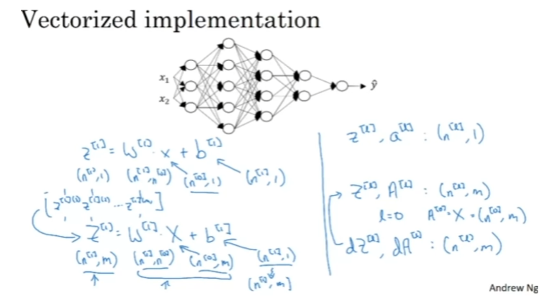
implementation. Previously we had z^ [1] equals w^ [1] times x plus b^ ]1], where this was n^ [1] by 1. This was n^ [1] by n^ [0], x was n^ [0] by 1, and b was n^ [1] by 1. Now, in a vectorized
implementation, you would have z^ [1] equals
w^ [1] times x plus b^ [1]. Where now z^ [1] is obtained by taking the z^ [1] for the
individual examples. So there’s z^ [1][1],
z^ [1][2] up to z^ [1][m] and stacking them as follows
and this gives you z^ [1]. The dimension of z^ [1] is that instead of being n^ [1] by 1, it ends up being n^ [1] by m, if m is decisive training set. The dimensions of
w^ [1] stays the same so is the n^ [1] by n^ [0] and x instead of being n^ [0] by 1 is now all your training
examples stamped horizontally, so it’s now n^ [0] by m. You
notice that when you take a, n^ [1] by n^ [0] matrics and multiply that by an
n^ 0] by m matrics that together they
actually give you an n^ [1] by m dimensional
matrics as expected. Now the final detail is that
b^ [1] is still n^ [1] by 1. But when you take
this and add it to b, then through python broadcasting
this will get duplicated into an n^ [1] by m matrics
and then added element-wise. On the previous slide, we talked about the
dimensions of w, b, dw, and db. Here what we see is
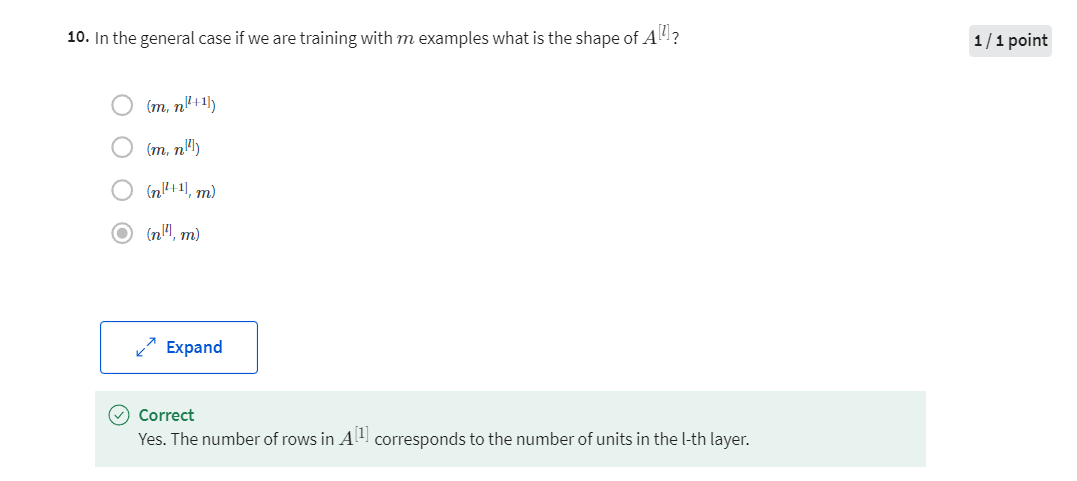
that whereas z^ [l], as well as a^ [l], are of dimension n^ [l] by 1, we have now instead
that capital Z^ [l], as well as capital A^ [l], are n^ [l] by m. A special case of this
is when l is equal to 0, in which case A^ [0], which is equal to
just your training set input features x is going to be equal to n^ [0]
by m as expected. Of course, when you’re implementing this in
back-propagation, we’ll see later you end up
computing dz as well as da. This way, of course, has the
same dimension as z and a. Hope the low exercise
went through helps clarify the dimensions of the various matrices
you’ll be working with.

When you implement
back-propagation for a deep neural network, so long as you work through
your code and make sure that all the matrices or
dimensions are consistent, that will usually
help you go some ways towards eliminating some
class of possible bugs. I hope that exercise
for figuring out the dimensions of
the various matrices you’d be working
with is helpful. When you implement a deep neural network if you keep straight the dimensions of
these various matrices and vectors you’re working with, hopefully, that will
help you eliminate some class of possible bugs. It certainly helps me
get my code right. Next, we’ve now seen
some of the mechanics of how to do the forward
propagation in a neural network. But why are deep neural
networks so effective and why do they do better than
shallow representations? Let’s spend a few minutes in
the next video to discuss.

Why Deep Representations?

We’ve all been hearing that deep
neural networks work really well for a lot of problems, and it’s not just that
they need to be big neural networks, is that specifically, they need to be
deep or to have a lot of hidden layers. So why is that? Let’s go through a couple examples and
try to gain some intuition for why deep networks might work well.

face recognition or face detection

So first,
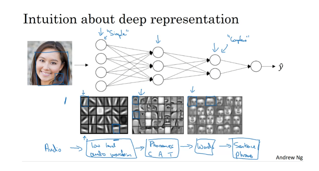
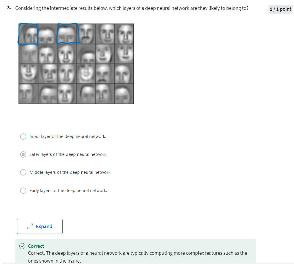
what is a deep network computing? If you’re building a system for
face recognition or face detection, here’s what a deep
neural network could be doing. Perhaps you input a picture of a face then
the first layer of the neural network you can think of as maybe being
a feature detector or an edge detector. In this example, I’m plotting what a
neural network with maybe 20 hidden units, might be trying to compute on this image. So the 20 hidden units visualized
by these little square boxes. So for example, this little visualization
represents a hidden unit that’s trying to figure out where the edges
of that orientation are in the image.

And maybe this hidden unit
might be trying to figure out where are the horizontal
edges in this image. And when we talk about convolutional
networks in a later course, this particular visualization
will make a bit more sense. But the form, you can think of the first layer
of the neural network as looking at the picture and trying to figure out
where are the edges in this picture. Now, let’s think about where the edges
in this picture by grouping together pixels to form edges. It can then detect the edges and group
edges together to form parts of faces. So for example, you might have a low
neuron trying to see if it’s finding an eye, or a different neuron trying
to find that part of the nose. And so by putting together lots of edges, it can start to detect
different parts of faces. And then, finally, by putting
together different parts of faces, like an eye or a nose or an ear or
a chin, it can then try to recognize or detect different types of faces. So intuitively, you can think of the
earlier layers of the neural network as detecting simple functions, like edges. And then composing them together in
the later layers of a neural network so that it can learn more and
more complex functions. These visualizations will make more sense
when we talk about convolutional nets. And one technical detail
of this visualization, the edge detectors are looking in
relatively small areas of an image, maybe very small regions like that. And then the facial detectors you can look
at maybe much larger areas of image. But the main intuition you take away
from this is just finding simple things like edges and then building them up. Composing them together to detect
more complex things like an eye or a nose then composing those together to
find even more complex things.

speech recognition system

And this type of simple to complex
hierarchical representation, or compositional representation, applies in other types of data than
images and face recognition as well. For example, if you’re trying to
build a speech recognition system, it’s hard to revisualize speech but if you input an audio clip then maybe
the first level of a neural network might learn to detect low level audio wave form
features, such as is this tone going up? Is it going down? Is it white noise or
sniffling sound like [SOUND]. And what is the pitch? When it comes to that, detect low
level wave form features like that. And then by composing
low level wave forms, maybe you’ll learn to detect
basic units of sound. In linguistics they call phonemes. But, for example, in the word cat,
the C is a phoneme, the A is a phoneme, the T is another phoneme. But learns to find maybe
the basic units of sound and then composing that together maybe
learn to recognize words in the audio. And then maybe compose those together, in order to recognize entire phrases or
sentences.

So deep neural network with multiple hidden
layers might be able to have the earlier layers learn these lower
level simple features and then have the later deeper layers then put
together the simpler things it’s detected in order to detect more complex things
like recognize specific words or even phrases or sentences. The uttering in order to
carry out speech recognition. And what we see is that whereas the other
layers are computing, what seems like relatively simple functions of the input
such as where the edge is, by the time you get deep in the network you can
actually do surprisingly complex things. Such as detect faces or
detect words or phrases or sentences.

Some people like to make an analogy
between deep neural networks and the human brain, where we believe,
or neuroscientists believe, that the human brain also starts off
detecting simple things like edges in what your eyes see then builds those
up to detect more complex things like the faces that you see. I think analogies between
deep learning and the human brain are sometimes
a little bit dangerous. But there is a lot of truth to, this being
how we think that human brain works and that the human brain probably
detects simple things like edges first then put them together to from more and
more complex objects and so that has served as a loose form of inspiration
for some deep learning as well. We’ll see a bit more
about the human brain or about the biological brain in
a later video this week.

circuit theory

The other piece of intuition
about why deep networks seem to work well is the following. So this result comes from circuit
theory of which pertains the thinking about what types of functions you can
compute with different AND gates, OR gates,
NOT gates, basically logic gates. So informally, their functions compute
with a relatively small but deep neural network and by small I mean the number
of hidden units is relatively small. But if you try to compute the same
function with a shallow network, so if there aren’t enough hidden layers, then you might require exponentially
more hidden units to compute. So let me just give you one example and
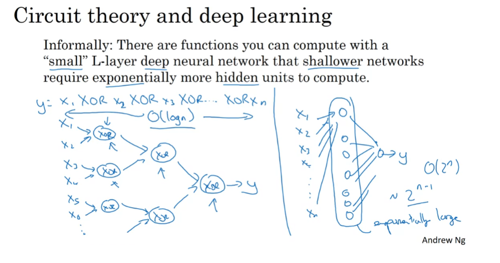
illustrate this a bit informally. But let’s say you’re trying to
compute the exclusive OR, or the parity of all your input features. So you’re trying to compute X1,
XOR, X2, XOR, X3, XOR, up to Xn if you have n or
n X features. So if you build in XOR tree like this,
so for us it computes the XOR of X1 and X2, then take X3 and
X4 and compute their XOR. And technically, if you’re just using
AND or NOT gate, you might need a couple layers to compute the XOR
function rather than just one layer, but with a relatively small circuit,
you can compute the XOR, and so on. And then you can build,
really, an XOR tree like so, until eventually, you have a circuit here
that outputs, well, lets call this Y. The outputs of Y hat equals Y. The exclusive OR,
the parity of all these input bits. So to compute XOR, the depth of the
network will be on the order of log N. We’ll just have an XOR tree. So the number of nodes or
the number of circuit components or the number of gates in this
network is not that large. You don’t need that many gates in
order to compute the exclusive OR.

But now, if you are not allowed to
use a neural network with multiple hidden layers with, in this case,
order log and hidden layers, if you’re forced to compute this
function with just one hidden layer, so you have all these things going into
the hidden units. And then these things then output Y. Then in order to compute this
XOR function, this hidden layer will need to be exponentially large,
because essentially, you need to exhaustively enumerate our
2 to the N possible configurations. So on the order of 2 to the N,
possible configurations of the input bits that result in the exclusive OR
being either 1 or 0. So you end up needing a hidden layer
that is exponentially large in the number of bits. I think technically, you could do this
with 2 to the N minus 1 hidden units. But that’s the older 2 to the N, so it’s going to
be exponentially larger on the number of bits. So I hope this gives a sense that
there are mathematical functions, that are much easier to compute with deep
networks than with shallow networks.

Actually, I personally found the result
from circuit theory less useful for gaining intuitions, but this is
one of the results that people often cite when explaining the value of
having very deep representations.

Now, in addition to this reasons for preferring deep neural networks,
to be perfectly honest, I think the other reasons the term deep
learning has taken off is just branding. This things just we call neural
networks with a lot of hidden layers, but the phrase deep learning is just
a great brand, it’s just so deep. So I think that once that term caught on
that really neural networks rebranded or neural networks with many
hidden layers rebranded, help to capture the popular
imagination as well. But regardless of the PR branding,
deep networks do work well.

Sometimes people go overboard and
insist on using tons of hidden layers. But when I’m starting out a new problem,
I’ll often really start out with even logistic regression then
try something with one or two hidden layers and
use that as a hyper parameter. Use that as a parameter or hyper parameter
that you tune in order to try to find the right depth for your neural network. But over the last several years there has
been a trend toward people finding that for some applications, very, very deep
neural networks here with maybe many dozens of layers sometimes, can sometimes
be the best model for a problem. So that’s it for the intuitions for
why deep learning seems to work well. Let’s now take a look at the mechanics
of how to implement not just front propagation, but also back propagation.

Building Blocks of Deep Neural Networks

In the earlier videos from this week, as well as from the videos
from the past several weeks, you’ve already seen the basic building
blocks of forward propagation and back propagation, the key components you
need to implement a deep neural network. Let’s see how you can put these components
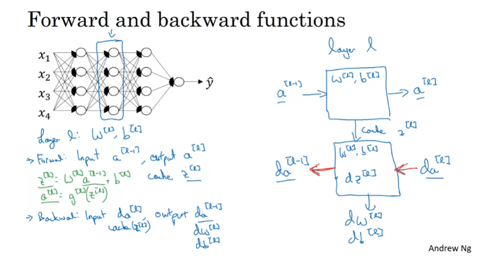
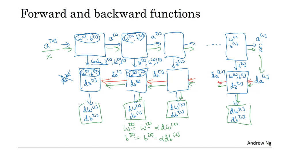
together to build your deep net. Here’s a network of a few layers. Let’s pick one layer. And look into the computations
focusing on just that layer for now. So for layer L,
you have some parameters wl and bl and for the forward prop, you will input the activations a l-1
from your previous layer and output a l. So the way we did this
previously was you compute z l = w l times al - 1 + b l. And then al = g of z l. All right. So, that’s how you go from the input
al minus one to the output al. And, it turns out that for later use it’ll
be useful to also cache the value zl. So, let me include this on cache as
well because storing the value zl would be useful for backward, for
the back propagation step later. And then for the backward step or for
the back propagation step, again, focusing on computation for this layer l, you’re going to implement
a function that inputs da(l). And outputs da(l-1), and
just to flesh out the details, the input is actually da(l),
as well as the cache so you have available to you the value
of zl that you computed and then in addition, outputing da(l)
minus 1 you bring the output or the gradients you want in order
to implement gradient descent for learning, okay? So this is the basic structure of
how you implement this forward step, what we call the forward function
as well as this backward step, which we’ll call backward function. So just to summarize, in layer l, you’re going to have the forward step or
the forward prop of the forward function. Input al- 1 and output, al, and in order to make this computation
you need to use wl and bl.

how you implement this forward step

And also output a cache,
which contains zl, right? And then the backward function,
using the back prop step, will be another function that now inputs da(l) and outputs da(l-1). So it tells you, given the derivatives
respect to these activations, that’s da(l), what are the derivatives? How much do I wish? You know, al- 1 changes the computed
derivatives respect to deactivations from a previous layer. Within this box, right? You need to use wl and bl, and
it turns out along the way you end up computing dzl, and then this box, this backward function
can also output dwl and dbl, but I was sometimes using red arrows
to denote the backward iteration. So if you prefer,
we could draw these arrows in red.

So if you can implement
these two functions then the basic computation of
the neural network will be as follows. You’re going to take the input
features a0, feed that in, and that would compute the activations of
the first layer, let’s call that a1 and to do that, you need a w1 and
b1 and then will also, you know, cache away z1, right? Now having done that, you feed that to
the second layer and then using w2 and b2, you’re going to compute deactivations
in the next layer a2 and so on. Until eventually, you end up outputting a l which is equal to y hat. And along the way,
we cached all of these values z. So that’s the forward propagation step. Now, for the back propagation step,
what we’re going to do will be a backward sequence of iterations in which you are going backwards and
computing gradients like so. So what you’re going to feed in here,
da(l) and then this box will give us da(l- 1) and
so on until we get da(2) da(1). You could actually get one more
output to compute da(0) but this is derivative with respect to your input features, which is
not useful at least for training the weights of these
supervised neural networks. So you could just stop it there. But
along the way, back prop also ends up outputting dwl,
dbl. I just used the prompt as wl and bl. This would output dw3, db3 and so on. So you end up computing all
the derivatives you need. And so just to maybe fill in
the structure of this a little bit more, these boxes will use
those parameters as well. wl, bl and it turns out that we’ll see later that inside these boxes
we end up computing the dz’s as well. So one iteration of training through
a neural network involves: starting with a(0) which is x and
going through forward prop as follows.

backward function

Computing y hat and
then using that to compute this and then back prop, right, doing that and now you have all these derivative
terms and so, you know, w would get updated as w1 =
the learning rate times dw, right? For each of the layers and
similarly for b rate. Now the computed back prop
have all these derivatives. So that’s one iteration of gradient
descent for your neural network. Now before moving on,
just one more informational detail. Conceptually, it will be useful
to think of the cache here as storing the value of z for
the backward functions. But when you implement this, and
you see this in the programming exercise, When you implement this,
you find that the cache may be a convenient way to get to this
value of the parameters of w1, b1, into the backward function as well.
So for this exercise you actually store in your
cache to z as well as w and b. So this stores z2, w2, b2.
But from an implementation standpoint, I just find it a convenient way
to just get the parameters, copy to where you need to use them later
when you’re computing back propagation. So that’s just an implementational
detail that you see when you do the programming exercise.

So you’ve now seen what
are the basic building blocks for implementing a deep neural network. In each layer there’s
a forward propagation step and there’s a corresponding
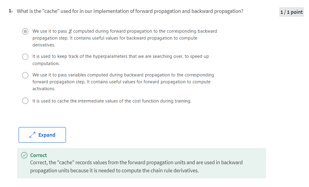
backward propagation step. And has a cache to pass
information from one to the other. In the next video, we’ll talk about how you can actually
implement these building blocks. Let’s go on to the next video.

Forward and Backward Propagation

forward propagation

In a previous video, you saw the basic blocks of implementing
a deep neural network, a forward propagation step for each layer and a corresponding
backward propagation step. Let’s see how you can actually
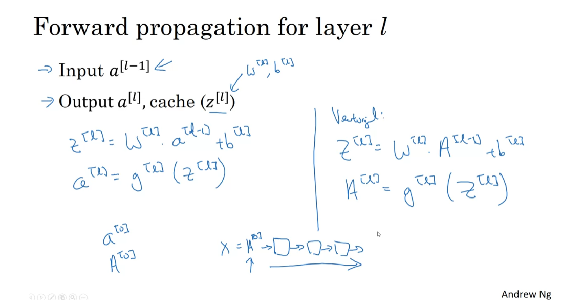
implement these steps. We’ll start with
forward propagation. Recall that what this will
do is input a^l minus 1, and outputs a^l and
the cache, z^l. We just said that, from
implementational point of view, maybe we’ll cache
w^l and b^l as well, just to make the
function’s call a bit easier in the
program exercise. The equations for this should
already look familiar. The way to implement a forward
function is just this, equals w^l times a^l
minus 1 plus b^l, and then a^l equals the
activation function applied to z. If you want a vectorized
implementation, then it’s just that times
a^l minus 1 plus b, b being a Python broadcasting, and a^l equals g, applied element-wise to z. You remember, on the
diagram for the 4th step, remember we had this chain
of boxes going forward, so you initialize
that with feeding in a^0, which is equal to x. So you initialize this with, what is the input
to the first one? It’s really a^0,
which is the input features either for
one training example if you’re doing one
example at a time, or a^0 if you’re processing
the entire training set. That’s the input to the first forward
function in the chain, and then just repeating
this allows you to compute forward propagation
from left to right.

backward propagation step

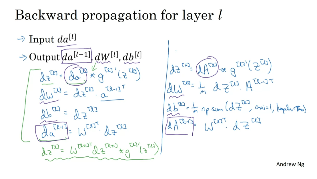
Next, let’s talk about the
backward propagation step. Here, your goal
is to input da^l, and output da^l minus
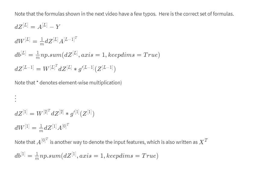
1 and dw^l and db^l. Let me just write out the steps you need to
compute these things. Dz^l is equal to da^l
element-wise product, with g of l prime z of l. Then to compute
the derivatives, dw^l equals dz^l
times a of l minus 1. I didn’t explicitly
put that in the cache, but it turns out you
need this as well. Then db^l is equal to
dz^l, and finally, da of l minus 1 is equal to w^l transpose times dz^l. I don’t want to go through the detailed
derivation for this, but it turns out that if
you take this definition for da and plug it in here, then you get the same formula as we had in there previously, for how you compute dz^l as a function of
the previous dz^l. In fact, well, if I
just plug that in here, you end up that dz^l is equal to w^l plus 1 transpose dz^l plus 1 times g^l prime z of l. I know this looks
like a lot of algebra. You could actually
double-check for yourself that this
is the equation we had written down for
back propagation last week, when we were doing
a neural network with just a single hidden layer. As a reminder, this times
is element-wise product, so all you need is those four equations to implement
your backward function.

vectorized version

Then finally, I’ll just write
out a vectorized version. So the first line becomes dz^l equals da^l element-wise
product with g^l prime of z^l, maybe no surprise there. Dw^l becomes 1 over m, dz^l times a^l
minus 1 transpose. Then db^l becomes 1
over m np.sum dz^l. Then axis equals 1,
keepdims equals true. We talked about the use of np.sum in the previous
week, to compute db. Then finally, da^l minus
1 is w^l transpose times dz of l. This allows you to input this
quantity, da, over here. Output dW^l, dp^l, the
derivatives you need, as well as da^l
minus 1 as follows. That’s how you implement
the backward function.

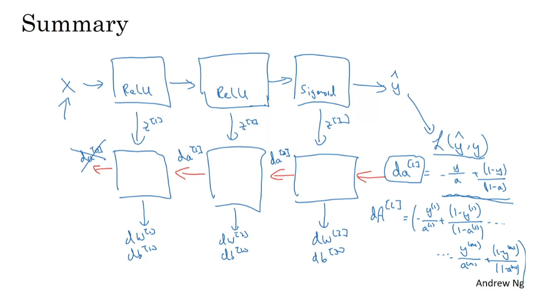
Just to summarize,
take the input x, you may have the
first layer maybe has a ReLU activation function. Then go to the second layer, maybe uses another ReLU
activation function, goes to the third
layer maybe has a sigmoid activation function if you’re doing binary
classification, and this outputs y-hat. Then using y-hat, you
can compute the loss. This allows you to start
your backward iteration. I’ll draw the arrows first. I guess I don’t have to
change pens too much. Where you will then have backprop compute
the derivatives, compute dW^3, db^3, dW^2, db^2, dW^1, db^1. Along the way you would be
computing against the cash. We’ll transfer z^1, z^2, z^3. Here you pass backwards
da^2 and da^1. This could compute da^0, but we won’t use that so
you can just discard that. This is how you implement
forward prop and back prop for a three-layer neural network.

There’s this one last
detail that I didn’t talk about which is for the
forward recursion, we will initialize it
with the input data x. How about the
backward recursion? Well it turns out that da of l when you’re using
logistic regression, when you’re doing
binary classification is equal to y over a plus 1 minus y over 1 minus a. It turns out that the derivative of the loss function respect to the output with respect to y-hat can be shown
to be what it is. If you’re familiar
with calculus, if you look up the
loss function l and take derivatives with respect
to y-hat with respect to a, you can show that you
get that formula. This is the formula
you should use for da, for the final layer, capital L.

Of course if you were to have a vectorized
implementation, then you initialize the backward recursion,
not with this, but with da capital A for the layer L which is going to be the same thing for the
different examples. Over a for the first train
example plus 1 minus y for the first
train example over 1 minus A for the
first train example, dot-dot-dot down to
the nth train example. So 1 minus a of M. That’s how you’d implement the
vectorized version. That’s how you initialize the vectorized version
of back propagation.

We’ve now seen the basic
building blocks of both forward propagation as
well as back propagation. Now if you implement
these equations, you will get the correct
implementation of forward prop and backprop to get you the
derivatives you need. You might be thinking, well
those are a lot of equations. I’m slightly confused.
I’m not quite sure I see how this works and if
you’re feeling that way, my advice is when you get to this week’s
programming assignment, you will be able to
implement these for yourself and they will
be much more concrete. I know those are a
lot of equations, and maybe some of the equations didn’t make complete sense, but if you work through the calculus and the linear
algebra which is not easy, so feel free to try, but that’s actually
one of the more difficult derivations
in machine learning. It turns out the equations
we wrote down are just the calculus equations for computing the derivatives, especially in backprop,
but once again, if this feels a
little bit abstract, a little bit mysterious to you, my advice is when you’ve done
the programming exercise, it will feel a bit
more concrete to you.

Although I have to say, even today when I implement
a learning algorithm, sometimes even I’m
surprised when my learning algorithm
implementation works and it’s because a lot of the complexity of machine learning comes from the data rather than
from the lines of codes. Sometimes you feel like you implement a
few lines of code, not quite sure what it did, but it almost magically works, and it’s because a lot of
magic is actually not in the piece of code you write
which is often not too long. It’s not exactly simple, but it’s not 10,000, 100,000 lines of code, but you feed it
so much data that sometimes even though I’ve worked with machine
learning for a long time, sometimes it still surprises me a bit when my learning
algorithm works, because a lot of
the complexity of your learning algorithm
comes from the data rather than necessarily from you writing thousands and
thousands of lines of code.

That’s how you implement
deep neural networks. Again this will become more concrete when you’ve done
the programming exercising. Before moving on,
in the next video, I want to discuss
hyper-parameters and parameters. It turns out that when
you’re training deep nets, being able to organize
your hyper-parameters well will help you be more efficient in developing your networks. In the next video, let’s talk about exactly what that means.

Optional Reading: Feedforward Neural Networks in Depth

For a more in depth explaination of Feedforward Neural Networks, one of our DLS mentors has written some articles (optional reading) on them. If these interest you, do check them out.

A huge shoutout and thanks to Jonas Lalin!

Parameters vs Hyperparameters

Being effective in developing your deep Neural Nets requires that you not only organize your parameters well but also your hyper parameters. So what are hyper parameters? let’s take a look!

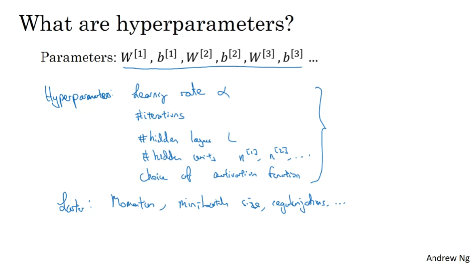
So the parameters your model are W and B and there are other things you need to tell your learning algorithm, such as the learning rate alpha, because we need to set alpha and that in turn will determine how your parameters evolve or maybe the number of iterations of gradient descent you carry out. Your learning algorithm has oth numbers that you need to set such as the number of hidden layers, so we call that capital L, or the number of hidden units, such as 0 and 1 and 2 and so on. Then you also have the choice of activation function. do you want to use a RELU, or tangent or a sigmoid function especially in the hidden layers. So all of these things are things that you need to tell your learning algorithm and so these are parameters that control the ultimate parameters W and B and so we call all of these things below hyper parameters.

hyper parameters

Because these things like alpha, the learning rate, the number of iterations, number of hidden layers, and so on, these are all parameters that control W and B. So we call these things hyper parameters, because it is the hyper parameters that somehow determine the final value of the parameters W and B that you end up with. In fact, deep learning has a lot of different hyper parameters.

In the later course, we’ll see other hyper parameters as well such as the momentum term, the mini batch size, various forms of regularization parameters, and so on. If none of these terms at the bottom make sense yet, don’t worry about it! We’ll talk about them in the second course.

Because deep learning has so many hyper parameters in contrast to earlier errors of machine learning, I’m going to try to be very consistent in calling the learning rate alpha a hyper parameter rather than calling the parameter. I think in earlier eras of machine learning when we didn’t have so many hyper parameters, most of us used to be a bit slow up here and just call alpha a parameter.

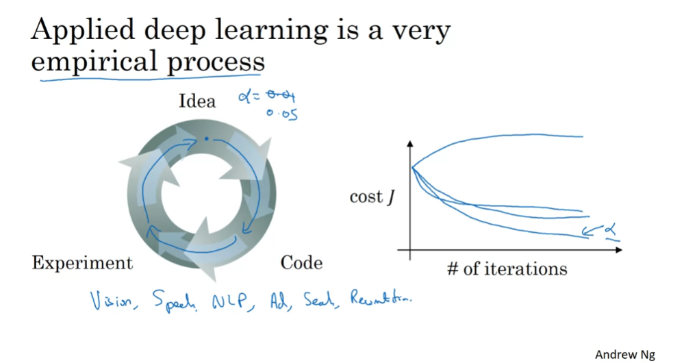
Technically, alpha is a parameter, but is a parameter that determines the real parameters. I’ll try to be consistent in calling these things like alpha, the number of iterations, and so on hyper parameters. So when you’re training a deep net for your own application you find that there may be a lot of possible settings for the hyper parameters that you need to just try out. So applying deep learning today is a very intrictate process where often you might have an idea. For example, you might have an idea for the best value for the learning rate. You might say, well maybe alpha equals 0.01 I want to try that. Then you implement, try it out, and then see how that works. Based on that outcome you might say, you know what? I’ve changed online, I want to increase the learning rate to 0.05. So, if you’re not sure what the best value for the learning rate to use. You might try one value of the learning rate alpha and see their cost function j go down like this, then you might try a larger value for the learning rate alpha and see the cost function blow up and diverge. Then, you might try another version and see it go down really fast. it’s inverse to higher value. You might try another version and see the cost function J do that then. I’ll be trying to set the values. So you might say, okay looks like this the value of alpha. It gives me a pretty fast learning and allows me to converge to a lower cost function j and so I’m going to use this value of alpha.

You saw in a previous slide that there are a lot of different hybrid parameters. It turns out that when you’re starting on the new application, you should find it very difficult to know in advance exactly what is the best value of the hyper parameters. So, what often happens is you just have to try out many different values and go around this cycle your try out some values, really try five hidden layers. With this many number of hidden units implement that, see if it works, and then iterate. So the title of this slide is that applying deep learning is a very empirical process, and empirical process is maybe a fancy way of saying you just have to try a lot of things and see what works.

Another effect I’ve seen is that deep learning today is applied to so many problems ranging from computer vision, to speech recognition, to natural language processing, to a lot of structured data applications such as maybe a online advertising, or web search, or product recommendations, and so on. What I’ve seen is that first, I’ve seen researchers from one discipline, any one of these, and try to go to a different one. And sometimes the intuitions about hyper parameters carries over and sometimes it doesn’t, so I often advise people, especially when starting on a new problem, to just try out a range of values and see what w. In the next course we’ll see some systematic ways for trying out a range of values. Second, even if you’re working on one application for a long time, you know maybe you’re working on online advertising, as you make progress on the problem it is quite possible that the best value for the learning rate, a number of hidden units, and so on might change.

So even if you tune your system to the best value of hyper parameters today it’s possible you’ll find that the best value might change a year from now maybe because the computer infrastructure, be it you know CPUs, or the type of GPU running on, or something has changed. So maybe one rule of thumb is every now and then, maybe every few months, if you’re working on a problem for an extended period of time for many years just try a few values for the hyper parameters and double check if there’s a better value for the hyper parameters. As you do so you slowly gain intuition as well about the hyper parameters that work best for your problems. I know that this might seem like an unsatisfying part of deep learning that you just have to try on all the values for these hyper parameters, but maybe this is one area where deep learning research is still advancing, and maybe over time we’ll be able to give better guidance for the best hyper parameters to use. It’s also possible that because CPUs and GPUs and networks and data sets are all changing, and it is possible that the guidance won’t converge for some time. You just need to keep trying out different values and evaluate them on a hold on cross-validation set or something and pick the value that works for your problems.

So that was a brief discussion of hyper parameters. In the second course, we’ll also give some suggestions for how to systematically explore the space of hyper parameters but by now you actually have pretty much all the tools you need to do their programming exercise before you do that adjust or share view one more set of ideas which is I often ask what does deep learning have to do the human brain?

Clarification For: What does this have to do with the brain?

What does this have to do with the brain?

So what does deep learning
have to do with the brain? At the risk of giving away the punchline I would
say, not a whole lot, but let’s take a quick look
at why people keep making the analogy between deep
learning and the human brain. When you implement
a neural network, this is what you do, forward prop and back prop. I think because it’s
been difficult to convey intuitions about what
these equations are doing, really creating the sense
on a very complex function, the analogy that it’s
like the brain has become an oversimplified
explanation for what this is doing.

But the simplicity of
this makes it seductive for people to just say it publicly as well as for
media to report it, and it is certainly called
the popular imagination. There is a very loose
analogy between, let’s say, a logistic regression unit with a sigmoid
activation function. Here’s a cartoon of a
single neuron in the brain. In this picture of a biological
neuron, this neuron, which is a cell in your brain, receives electric signals
from other neurons, X1, X2, X3, or maybe from
other neurons, A1, A2, A3, does a simple
thresholding computation, and then if this neuron fires, it sends a pulse of
electricity down the axon, down this long wire, perhaps to other neurons. There is a very
simplistic analogy between a single neuron
in a neural network, and a biological neuron like
that shown on the right.

But I think that today
even neuroscientists have almost no idea what even
a single neuron is doing. A single neuron appears
to be much more complex than we are able to
characterize with neuroscience, and while some of what it’s doing is a little bit
like logistic regression, there’s still a lot about
what even a single neuron does that no one human
today understands. For example, exactly
how neurons in the human brain learns is still a very mysterious process, and it’s completely
unclear today whether the human brain
uses an algorithm, does anything like
back propagation or gradient descent
or if there’s some fundamentally different
learning principle that the human brain uses. When I think of deep-learning, I think of it as being very good and learning very
flexible functions, very complex functions,
to learn X to Y mappings, to learn input-output mappings
in supervised learning. Whereas this is like
the brain analogy, maybe that was useful once, I think the field has moved to the point where that
analogy is breaking down, and I tend not to use that
analogy much anymore.

So that’s it for neural
networks and the brain. I do think that
maybe the field of computer vision has taken a bit more inspiration
from the human brain than other disciplines that
also apply deep learning, but I personally use the analogy to the human
brain less than I used to. That’s it for this video. You now know how to implement
forward prop and back prop and gradient descent even
for deep neural networks. Best of luck with the
programming exercise, and I look forward
to sharing more of these ideas with you
in the second course.

Quiz: Key Concepts on Deep Neural Networks

Programming Assignment: Building your Deep Neural Network: Step by Step

Building your Deep Neural Network: Step by Step

Welcome to your week 4 assignment (part 1 of 2)! Previously you trained a 2-layer Neural Network with a single hidden layer. This week, you will build a deep neural network with as many layers as you want!

• In this notebook, you’ll implement all the functions required to build a deep neural network.
• For the next assignment, you’ll use these functions to build a deep neural network for image classification.

By the end of this assignment, you’ll be able to:

• Use non-linear units like ReLU to improve your model
• Build a deeper neural network (with more than 1 hidden layer)
• Implement an easy-to-use neural network class

Notation:

• Superscript $[l]$ denotes a quantity associated with the $l^{th}$ layer.
  • Example: $a^{[L]}$ is the $L^{th}$ layer activation. $W^{[L]}$ and $b^{[L]}$ are the $L^{th}$ layer parameters.
• Superscript $(i)$ denotes a quantity associated with the $i^{th}$ example.
  • Example: $x^{(i)}$ is the $i^{th}$ training example.
• Lowerscript $i$ denotes the $i^{th}$ entry of a vector.
  • Example: $a_i^{[l]}$ denotes the $i^{th}$ entry of the $l^{th}$ layer’s activations).

Let’s get started!

Important Note on Submission to the AutoGrader

Before submitting your assignment to the AutoGrader, please make sure you are not doing the following:

1. You have not added any extra print statement(s) in the assignment.
2. You have not added any extra code cell(s) in the assignment.
3. You have not changed any of the function parameters.
4. You are not using any global variables inside your graded exercises. Unless specifically instructed to do so, please refrain from it and use the local variables instead.
5. You are not changing the assignment code where it is not required, like creating extra variables.

If you do any of the following, you will get something like, Grader Error: Grader feedback not found (or similarly unexpected) error upon submitting your assignment. Before asking for help/debugging the errors in your assignment, check for these first. If this is the case, and you don’t remember the changes you have made, you can get a fresh copy of the assignment by following these instructions.

1 - Packages

First, import all the packages you’ll need during this assignment.

• numpy is the main package for scientific computing with Python.
• matplotlib is a library to plot graphs in Python.
• dnn_utils provides some necessary functions for this notebook.
• testCases provides some test cases to assess the correctness of your functions
• np.random.seed(1) is used to keep all the random function calls consistent. It helps grade your work. Please don’t change the seed!

import numpy as np
import h5py
import matplotlib.pyplot as plt
from testCases import *
from dnn_utils import sigmoid, sigmoid_backward, relu, relu_backward
from public_tests import *

import copy
%matplotlib inline
plt.rcParams['figure.figsize'] = (5.0, 4.0) # set default size of plots
plt.rcParams['image.interpolation'] = 'nearest'
plt.rcParams['image.cmap'] = 'gray'

%load_ext autoreload
%autoreload 2

np.random.seed(1)

dnn_utils.py文件如下：

import numpy as np

def sigmoid(Z):
    """
    Implements the sigmoid activation in numpy
    
    Arguments:
    Z -- numpy array of any shape
    
    Returns:
    A -- output of sigmoid(z), same shape as Z
    cache -- returns Z as well, useful during backpropagation
    """
    
    A = 1/(1+np.exp(-Z))
    cache = Z
    
    return A, cache

def relu(Z):
    """
    Implement the RELU function.

    Arguments:
    Z -- Output of the linear layer, of any shape

    Returns:
    A -- Post-activation parameter, of the same shape as Z
    cache -- a python dictionary containing "A" ; stored for computing the backward pass efficiently
    """
    
    A = np.maximum(0,Z)
    
    assert(A.shape == Z.shape)
    
    cache = Z 
    return A, cache


def relu_backward(dA, cache):
    """
    Implement the backward propagation for a single RELU unit.

    Arguments:
    dA -- post-activation gradient, of any shape
    cache -- 'Z' where we store for computing backward propagation efficiently

    Returns:
    dZ -- Gradient of the cost with respect to Z
    """
    
    Z = cache
    dZ = np.array(dA, copy=True) # just converting dz to a correct object.
    
    # When z <= 0, you should set dz to 0 as well. 
    dZ[Z <= 0] = 0
    
    assert (dZ.shape == Z.shape)
    
    return dZ

def sigmoid_backward(dA, cache):
    """
    Implement the backward propagation for a single SIGMOID unit.

    Arguments:
    dA -- post-activation gradient, of any shape
    cache -- 'Z' where we store for computing backward propagation efficiently

    Returns:
    dZ -- Gradient of the cost with respect to Z
    """
    
    Z = cache
    
    s = 1/(1+np.exp(-Z))
    dZ = dA * s * (1-s)
    
    assert (dZ.shape == Z.shape)
    
    return dZ

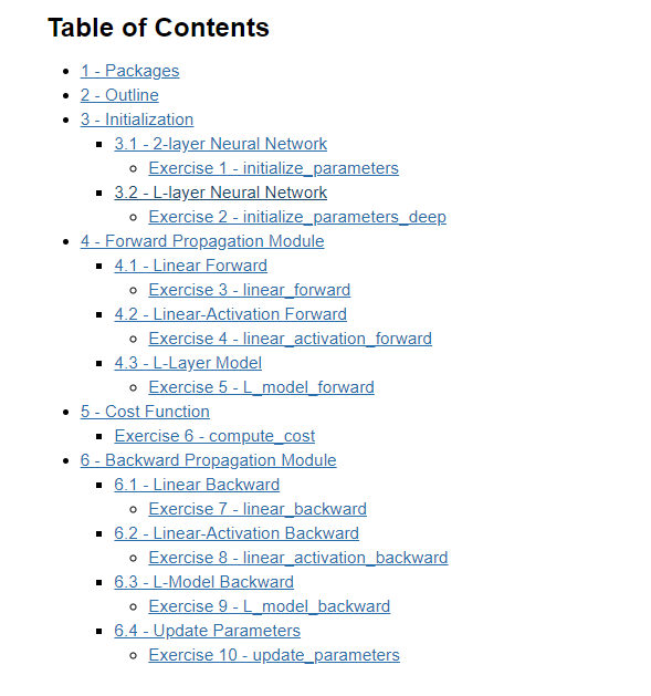
2 - Outline

To build your neural network, you’ll be implementing several “helper functions.” These helper functions will be used in the next assignment to build a two-layer neural network and an L-layer neural network.

Each small helper function will have detailed instructions to walk you through the necessary steps. Here’s an outline of the steps in this assignment:

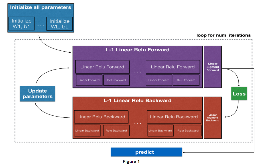
• Initialize the parameters for a two-layer network and for an $L$-layer neural network
• Implement the forward propagation module (shown in purple in the figure below)
  • Complete the LINEAR part of a layer’s forward propagation step (resulting in $Z^{[l]}$).
  • The ACTIVATION function is provided for you (relu/sigmoid)
  • Combine the previous two steps into a new [LINEAR->ACTIVATION] forward function.
  • Stack the [LINEAR->RELU] forward function L-1 time (for layers 1 through L-1) and add a [LINEAR->SIGMOID] at the end (for the final layer $L$). This gives you a new L_model_forward function.
• Compute the loss
• Implement the backward propagation module (denoted in red in the figure below)
  • Complete the LINEAR part of a layer’s backward propagation step
  • The gradient of the ACTIVATION function is provided for you(relu_backward/sigmoid_backward)
  • Combine the previous two steps into a new [LINEAR->ACTIVATION] backward function
  • Stack [LINEAR->RELU] backward L-1 times and add [LINEAR->SIGMOID] backward in a new L_model_backward function
• Finally, update the parameters

Figure 1

Note:

For every forward function, there is a corresponding backward function. This is why at every step of your forward module you will be storing some values in a cache. These cached values are useful for computing gradients.

In the backpropagation module, you can then use the cache to calculate the gradients. Don’t worry, this assignment will show you exactly how to carry out each of these steps!

3 - Initialization

You will write two helper functions to initialize the parameters for your model. The first function will be used to initialize parameters for a two layer model. The second one generalizes this initialization process to $L$ layers.

3.1 - 2-layer Neural Network

Exercise 1 - initialize_parameters

Create and initialize the parameters of the 2-layer neural network.

Instructions:

• The model’s structure is: LINEAR -> RELU -> LINEAR -> SIGMOID.
• Use this random initialization for the weight matrices: np.random.randn(d0, d1, ..., dn) * 0.01 with the correct shape. The documentation for np.random.randn
• Use zero initialization for the biases: np.zeros(shape). The documentation for np.zeros

# GRADED FUNCTION: initialize_parameters

def initialize_parameters(n_x, n_h, n_y):
    """
    Argument:
    n_x -- size of the input layer
    n_h -- size of the hidden layer
    n_y -- size of the output layer
    
    Returns:
    parameters -- python dictionary containing your parameters:
                    W1 -- weight matrix of shape (n_h, n_x)
                    b1 -- bias vector of shape (n_h, 1)
                    W2 -- weight matrix of shape (n_y, n_h)
                    b2 -- bias vector of shape (n_y, 1)
    """
    
    np.random.seed(1)
    
    #(≈ 4 lines of code)
    # W1 = ...
    # b1 = ...
    # W2 = ...
    # b2 = ...
    # YOUR CODE STARTS HERE
    W1 = np.random.randn(n_h, n_x) * 0.01
    b1 = np.zeros((n_h, 1))
    W2 = np.random.randn(n_y, n_h) * 0.01
    b2 = np.zeros((n_y, 1))
    
    # YOUR CODE ENDS HERE
    
    parameters = {"W1": W1,
                  "b1": b1,
                  "W2": W2,
                  "b2": b2}
    
    return parameters    

print("Test Case 1:\n")
parameters = initialize_parameters(3,2,1)

print("W1 = " + str(parameters["W1"]))
print("b1 = " + str(parameters["b1"]))
print("W2 = " + str(parameters["W2"]))
print("b2 = " + str(parameters["b2"]))

initialize_parameters_test_1(initialize_parameters)

print("\033[90m\nTest Case 2:\n")
parameters = initialize_parameters(4,3,2)

print("W1 = " + str(parameters["W1"]))
print("b1 = " + str(parameters["b1"]))
print("W2 = " + str(parameters["W2"]))
print("b2 = " + str(parameters["b2"]))

initialize_parameters_test_2(initialize_parameters)

Output

Test Case 1:

W1 = [[ 0.01624345 -0.00611756 -0.00528172]
 [-0.01072969  0.00865408 -0.02301539]]
b1 = [[0.]
 [0.]]
W2 = [[ 0.01744812 -0.00761207]]
b2 = [[0.]]
 All tests passed.

Test Case 2:

W1 = [[ 0.01624345 -0.00611756 -0.00528172 -0.01072969]
 [ 0.00865408 -0.02301539  0.01744812 -0.00761207]
 [ 0.00319039 -0.0024937   0.01462108 -0.02060141]]
b1 = [[0.]
 [0.]
 [0.]]
W2 = [[-0.00322417 -0.00384054  0.01133769]
 [-0.01099891 -0.00172428 -0.00877858]]
b2 = [[0.]
 [0.]]
 All tests passed.

Expected output

Test Case 1:

W1 = [[ 0.01624345 -0.00611756 -0.00528172]
 [-0.01072969  0.00865408 -0.02301539]]
b1 = [[0.]
 [0.]]
W2 = [[ 0.01744812 -0.00761207]]
b2 = [[0.]]
 All tests passed.

Test Case 2:

W1 = [[ 0.01624345 -0.00611756 -0.00528172 -0.01072969]
 [ 0.00865408 -0.02301539  0.01744812 -0.00761207]
 [ 0.00319039 -0.0024937   0.01462108 -0.02060141]]
b1 = [[0.]
 [0.]
 [0.]]
W2 = [[-0.00322417 -0.00384054  0.01133769]
 [-0.01099891 -0.00172428 -0.00877858]]
b2 = [[0.]
 [0.]]
 All tests passed.

3.2 - L-layer Neural Network

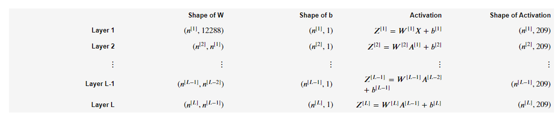
The initialization for a deeper L-layer neural network is more complicated because there are many more weight matrices and bias vectors. When completing the initialize_parameters_deep function, you should make sure that your dimensions match between each layer. Recall that $n^{[l]}$ is the number of units in layer $l$. For example, if the size of your input $X$ is $(12288,209)$ (with $m=209$ examples) then:

Remember that when you compute $WX+b$ in python, it carries out broadcasting. For example, if:

$$W=\left[\begin{array}{ccc}{w}_{00}& w_{01}& w_{02}\\ w_{10}& w_{11}& w_{12}\\ w_{20}& w_{21}& w_{22}\end{array}\right]X=\left[\begin{array}{ccc}{x}_{00}& x_{01}& x_{02}\\ x_{10}& x_{11}& x_{12}\\ x_{20}& x_{21}& x_{22}\end{array}\right]b=\left[\begin{array}{c}{b}_0\\ b_1\\ b_2\end{array}\right]\text{\hspace{1em}(2)}$$

Then $WX+b$ will be:

$$WX+b=\left[\begin{array}{ccc}(w_{00}{x}_{00}+w_{01}{x}_{10}+w_{02}{x}_{20})+b_0& (w_{00}{x}_{01}+w_{01}{x}_{11}+w_{02}{x}_{21})+b_0& \cdots \\ (w_{10}{x}_{00}+w_{11}{x}_{10}+w_{12}{x}_{20})+b_1& (w_{10}{x}_{01}+w_{11}{x}_{11}+w_{12}{x}_{21})+b_1& \cdots \\ (w_{20}{x}_{00}+w_{21}{x}_{10}+w_{22}{x}_{20})+b_2& (w_{20}{x}_{01}+w_{21}{x}_{11}+w_{22}{x}_{21})+b_2& \cdots \end{array}\right]\text{\hspace{1em}(3)}$$

Exercise 2 - initialize_parameters_deep

Implement initialization for an L-layer Neural Network.

Instructions:

• The model’s structure is [LINEAR -> RELU] $ \times$ (L-1) -> LINEAR -> SIGMOID. I.e., it has $L-1$ layers using a ReLU activation function followed by an output layer with a sigmoid activation function.
• Use random initialization for the weight matrices. Use np.random.randn(d0, d1, ..., dn) * 0.01.
• Use zeros initialization for the biases. Use np.zeros(shape).
• You’ll store $n^{[l]}$, the number of units in different layers, in a variable layer_dims. For example, the layer_dims for last week’s Planar Data classification model would have been [2,4,1]: There were two inputs, one hidden layer with 4 hidden units, and an output layer with 1 output unit. This means W1’s shape was (4,2), b1 was (4,1), W2 was (1,4) and b2 was (1,1). Now you will generalize this to $L$ layers!
• Here is the implementation for $L=1$ (one layer neural network). It should inspire you to implement the general case (L-layer neural network).

    if L == 1:
        parameters["W" + str(L)] = np.random.randn(layer_dims[1], layer_dims[0]) * 0.01
        parameters["b" + str(L)] = np.zeros((layer_dims[1], 1))

# GRADED FUNCTION: initialize_parameters_deep

def initialize_parameters_deep(layer_dims):
    """
    Arguments:
    layer_dims -- python array (list) containing the dimensions of each layer in our network
    
    Returns:
    parameters -- python dictionary containing your parameters "W1", "b1", ..., "WL", "bL":
                    Wl -- weight matrix of shape (layer_dims[l], layer_dims[l-1])
                    bl -- bias vector of shape (layer_dims[l], 1)
    """
    
    np.random.seed(3)
    parameters = {}
    L = len(layer_dims) # number of layers in the network

    for l in range(1, L):
        #(≈ 2 lines of code)
        # parameters['W' + str(l)] = ...
        # parameters['b' + str(l)] = ...
        # YOUR CODE STARTS HERE
        parameters["W" + str(l)] = np.random.randn(layer_dims[l], layer_dims[l-1]) * 0.01
        parameters["b" + str(l)] = np.zeros((layer_dims[l], 1))
        
        # YOUR CODE ENDS HERE
        
        assert(parameters['W' + str(l)].shape == (layer_dims[l], layer_dims[l - 1]))
        assert(parameters['b' + str(l)].shape == (layer_dims[l], 1))

        
    return parameters

print("Test Case 1:\n")
parameters = initialize_parameters_deep([5,4,3])

print("W1 = " + str(parameters["W1"]))
print("b1 = " + str(parameters["b1"]))
print("W2 = " + str(parameters["W2"]))
print("b2 = " + str(parameters["b2"]))

initialize_parameters_deep_test_1(initialize_parameters_deep)

print("\033[90m\nTest Case 2:\n")
parameters = initialize_parameters_deep([4,3,2])

print("W1 = " + str(parameters["W1"]))
print("b1 = " + str(parameters["b1"]))
print("W2 = " + str(parameters["W2"]))
print("b2 = " + str(parameters["b2"]))
initialize_parameters_deep_test_2(initialize_parameters_deep)

Output

Test Case 1:

W1 = [[ 0.01788628  0.0043651   0.00096497 -0.01863493 -0.00277388]
 [-0.00354759 -0.00082741 -0.00627001 -0.00043818 -0.00477218]
 [-0.01313865  0.00884622  0.00881318  0.01709573  0.00050034]
 [-0.00404677 -0.0054536  -0.01546477  0.00982367 -0.01101068]]
b1 = [[0.]
 [0.]
 [0.]
 [0.]]
W2 = [[-0.01185047 -0.0020565   0.01486148  0.00236716]
 [-0.01023785 -0.00712993  0.00625245 -0.00160513]
 [-0.00768836 -0.00230031  0.00745056  0.01976111]]
b2 = [[0.]
 [0.]
 [0.]]
 All tests passed.

Test Case 2:

W1 = [[ 0.01788628  0.0043651   0.00096497 -0.01863493]
 [-0.00277388 -0.00354759 -0.00082741 -0.00627001]
 [-0.00043818 -0.00477218 -0.01313865  0.00884622]]
b1 = [[0.]
 [0.]
 [0.]]
W2 = [[ 0.00881318  0.01709573  0.00050034]
 [-0.00404677 -0.0054536  -0.01546477]]
b2 = [[0.]
 [0.]]
 All tests passed.

Expected output

Test Case 1:

W1 = [[ 0.01788628  0.0043651   0.00096497 -0.01863493 -0.00277388]
 [-0.00354759 -0.00082741 -0.00627001 -0.00043818 -0.00477218]
 [-0.01313865  0.00884622  0.00881318  0.01709573  0.00050034]
 [-0.00404677 -0.0054536  -0.01546477  0.00982367 -0.01101068]]
b1 = [[0.]
 [0.]
 [0.]
 [0.]]
W2 = [[-0.01185047 -0.0020565   0.01486148  0.00236716]
 [-0.01023785 -0.00712993  0.00625245 -0.00160513]
 [-0.00768836 -0.00230031  0.00745056  0.01976111]]
b2 = [[0.]
 [0.]
 [0.]]
 All tests passed.

Test Case 2:

W1 = [[ 0.01788628  0.0043651   0.00096497 -0.01863493]
 [-0.00277388 -0.00354759 -0.00082741 -0.00627001]
 [-0.00043818 -0.00477218 -0.01313865  0.00884622]]
b1 = [[0.]
 [0.]
 [0.]]
W2 = [[ 0.00881318  0.01709573  0.00050034]
 [-0.00404677 -0.0054536  -0.01546477]]
b2 = [[0.]
 [0.]]
 All tests passed.

4 - Forward Propagation Module

4.1 - Linear Forward

Now that you have initialized your parameters, you can do the forward propagation module. Start by implementing some basic functions that you can use again later when implementing the model. Now, you’ll complete three functions in this order:

• LINEAR
• LINEAR -> ACTIVATION where ACTIVATION will be either ReLU or Sigmoid.
• [LINEAR -> RELU] $\times$ (L-1) -> LINEAR -> SIGMOID (whole model)

The linear forward module (vectorized over all the examples) computes the following equations:

$$Z^{[l]}=W^{[l]}{A}^{[l-1]}+b^{[l]}\text{\hspace{1em}(4)}$$

where $A^{[0]}=X$.

Exercise 3 - linear_forward

Build the linear part of forward propagation.

Reminder:
The mathematical representation of this unit is $Z^{[l]}=W^{[l]}{A}^{[l-1]}+b^{[l]}$. You may also find np.dot() useful. If your dimensions don’t match, printing W.shape may help.

# GRADED FUNCTION: linear_forward

def linear_forward(A, W, b):
    """
    Implement the linear part of a layer's forward propagation.

    Arguments:
    A -- activations from previous layer (or input data): (size of previous layer, number of examples)
    W -- weights matrix: numpy array of shape (size of current layer, size of previous layer)
    b -- bias vector, numpy array of shape (size of the current layer, 1)

    Returns:
    Z -- the input of the activation function, also called pre-activation parameter 
    cache -- a python tuple containing "A", "W" and "b" ; stored for computing the backward pass efficiently
    """
    
    #(≈ 1 line of code)
    # Z = ...
    # YOUR CODE STARTS HERE
    Z = np.dot(W, A) + b
    
    # YOUR CODE ENDS HERE
    cache = (A, W, b)
    
    return Z, cache

t_A, t_W, t_b = linear_forward_test_case()
t_Z, t_linear_cache = linear_forward(t_A, t_W, t_b)
print("Z = " + str(t_Z))

linear_forward_test(linear_forward)

Output

Z = [[ 3.26295337 -1.23429987]]
 All tests passed.

Expected output

Z = [[ 3.26295337 -1.23429987]]

4.2 - Linear-Activation Forward

In this notebook, you will use two activation functions:

• Sigmoid: $\sigma (Z)=\sigma (WA+b)=\frac{1}{1+e^{-(WA+b)}}$. You’ve been provided with the sigmoid function which returns two items: the activation value “a” and a “cache” that contains “Z” (it’s what we will feed in to the corresponding backward function). To use it you could just call:

A, activation_cache = sigmoid(Z)

• ReLU: The mathematical formula for ReLu is $A=RELU(Z)=max(0,Z)$. You’ve been provided with the relu function. This function returns two items: the activation value “A” and a “cache” that contains “Z” (it’s what you’ll feed in to the corresponding backward function). To use it you could just call:

A, activation_cache = relu(Z)

For added convenience, you’re going to group two functions (Linear and Activation) into one function (LINEAR->ACTIVATION). Hence, you’ll implement a function that does the LINEAR forward step, followed by an ACTIVATION forward step.

Exercise 4 - linear_activation_forward

Implement the forward propagation of the LINEAR->ACTIVATION layer. Mathematical relation is: $A^{[l]}=g(Z^{[l]})=g(W^{[l]}{A}^{[l-1]}+b^{[l]})$ where the activation “g” can be sigmoid() or relu(). Use linear_forward() and the correct activation function.

# GRADED FUNCTION: linear_activation_forward

def linear_activation_forward(A_prev, W, b, activation):
    """
    Implement the forward propagation for the LINEAR->ACTIVATION layer

    Arguments:
    A_prev -- activations from previous layer (or input data): (size of previous layer, number of examples)
    W -- weights matrix: numpy array of shape (size of current layer, size of previous layer)
    b -- bias vector, numpy array of shape (size of the current layer, 1)
    activation -- the activation to be used in this layer, stored as a text string: "sigmoid" or "relu"

    Returns:
    A -- the output of the activation function, also called the post-activation value 
    cache -- a python tuple containing "linear_cache" and "activation_cache";
             stored for computing the backward pass efficiently
    """
    
    if activation == "sigmoid":
        #(≈ 2 lines of code)
        # Z, linear_cache = ...
        # A, activation_cache = ...
        # YOUR CODE STARTS HERE
        Z, linear_cache = linear_forward(A_prev, W, b)
        A, activation_cache = sigmoid(Z)
        
        # YOUR CODE ENDS HERE
    
    elif activation == "relu":
        #(≈ 2 lines of code)
        # Z, linear_cache = ...
        # A, activation_cache = ...
        # YOUR CODE STARTS HERE
        Z, linear_cache = linear_forward(A_prev, W, b)
        A, activation_cache = relu(Z)
        
        # YOUR CODE ENDS HERE
    cache = (linear_cache, activation_cache)

    return A, cache

t_A_prev, t_W, t_b = linear_activation_forward_test_case()

t_A, t_linear_activation_cache = linear_activation_forward(t_A_prev, t_W, t_b, activation = "sigmoid")
print("With sigmoid: A = " + str(t_A))

t_A, t_linear_activation_cache = linear_activation_forward(t_A_prev, t_W, t_b, activation = "relu")
print("With ReLU: A = " + str(t_A))

linear_activation_forward_test(linear_activation_forward)

Output

With sigmoid: A = [[0.96890023 0.11013289]]
With ReLU: A = [[3.43896131 0.        ]]
 All tests passed.

Expected output

With sigmoid: A = [[0.96890023 0.11013289]]
With ReLU: A = [[3.43896131 0.        ]]

Note: In deep learning, the “[LINEAR->ACTIVATION]” computation is counted as a single layer in the neural network, not two layers.

4.3 - L-Layer Model

For even more convenience when implementing the $L$-layer Neural Net, you will need a function that replicates the previous one (linear_activation_forward with RELU) $L-1$ times, then follows that with one linear_activation_forward with SIGMOID.

Exercise 5 - L_model_forward

Implement the forward propagation of the above model.

Instructions: In the code below, the variable AL will denote $A^{[L]}=\sigma (Z^{[L]})=\sigma (W^{[L]}{A}^{[L-1]}+b^{[L]})$. (This is sometimes also called Yhat, i.e., this is $\hat{Y}$.)

Hints:

• Use the functions you’ve previously written
• Use a for loop to replicate [LINEAR->RELU] (L-1) times
• Don’t forget to keep track of the caches in the “caches” list. To add a new value c to a list, you can use list.append(c).

# GRADED FUNCTION: L_model_forward

def L_model_forward(X, parameters):
    """
    Implement forward propagation for the [LINEAR->RELU]*(L-1)->LINEAR->SIGMOID computation
    
    Arguments:
    X -- data, numpy array of shape (input size, number of examples)
    parameters -- output of initialize_parameters_deep()
    
    Returns:
    AL -- activation value from the output (last) layer
    caches -- list of caches containing:
                every cache of linear_activation_forward() (there are L of them, indexed from 0 to L-1)
    """

    caches = []
    A = X
    L = len(parameters) // 2                  # number of layers in the neural network
    
    # Implement [LINEAR -> RELU]*(L-1). Add "cache" to the "caches" list.
    # The for loop starts at 1 because layer 0 is the input
    for l in range(1, L):
        A_prev = A 
        #(≈ 2 lines of code)
        # A, cache = ...
        # caches ...
        # YOUR CODE STARTS HERE
        A, cache = linear_activation_forward(A_prev,  parameters["W" + str(l)],  parameters["b" + str(l)], activation="relu")
        caches.append(cache)
        
        # YOUR CODE ENDS HERE
    
    # Implement LINEAR -> SIGMOID. Add "cache" to the "caches" list.
    #(≈ 2 lines of code)
    # AL, cache = ...
    # caches ...
    # YOUR CODE STARTS HERE
    AL, cache = linear_activation_forward(A, parameters["W" + str(L)], parameters["b" + str(L)], activation="sigmoid")
    caches.append(cache)
    
    # YOUR CODE ENDS HERE
          
    return AL, caches

t_X, t_parameters = L_model_forward_test_case_2hidden()
t_AL, t_caches = L_model_forward(t_X, t_parameters)

print("AL = " + str(t_AL))

L_model_forward_test(L_model_forward)

Output

AL = [[0.03921668 0.70498921 0.19734387 0.04728177]]
 All tests passed.

Expected output

AL = [[0.03921668 0.70498921 0.19734387 0.04728177]]

Awesome! You’ve implemented a full forward propagation that takes the input X and outputs a row vector $A^{[L]}$ containing your predictions. It also records all intermediate values in “caches”. Using $A^{[L]}$, you can compute the cost of your predictions.

5 - Cost Function

Now you can implement forward and backward propagation! You need to compute the cost, in order to check whether your model is actually learning.

Exercise 6 - compute_cost

Compute the cross-entropy cost $J$, using the following formula: $$-\frac{1}{m}\sum _{i=1}^m(y^{(i)}\log \left(a^{[L](i)}\right)+(1-y^{(i)})\log \left(1-a^{[L](i)}\right))\text{\hspace{1em}(7)}$$

np.multiply 和 np.dot 是 NumPy 库中用于执行数组操作的两个不同的函数。

1. np.multiply：该函数执行的是元素级别的乘法，即将两个数组中对应位置的元素相乘。如果两个数组的形状不同，它会在执行操作之前进行广播。

import numpy as np

arr1 = np.array([1, 2, 3])
arr2 = np.array([4, 5, 6])

result = np.multiply(arr1, arr2)
print(result)  # 输出: [ 4 10 18]

2. np.dot：该函数执行的是矩阵乘法，它将第一个数组的行与第二个数组的列进行内积运算，得到一个新的数组。矩阵乘法要求第一个数组的列数等于第二个数组的行数。

import numpy as np

arr1 = np.array([[1, 2], [3, 4]])
arr2 = np.array([[5, 6], [7, 8]])

result = np.dot(arr1, arr2)
print(result)
# 输出:
# [[19 22]
#  [43 50]]

总结：

• np.multiply：用于执行元素级别的乘法。
• np.dot：用于执行矩阵乘法。

# GRADED FUNCTION: compute_cost

def compute_cost(AL, Y):
    """
    Implement the cost function defined by equation (7).

    Arguments:
    AL -- probability vector corresponding to your label predictions, shape (1, number of examples)
    Y -- true "label" vector (for example: containing 0 if non-cat, 1 if cat), shape (1, number of examples)

    Returns:
    cost -- cross-entropy cost
    """
    
    m = Y.shape[1]

    # Compute loss from aL and y.
    # (≈ 1 lines of code)
    # cost = ...
    # YOUR CODE STARTS HERE
    cost = - 1 / m * np.sum(np.multiply(Y, np.log(AL)) + np.multiply(1 - Y, np.log(1 - AL)))
    
    # YOUR CODE ENDS HERE
    
    cost = np.squeeze(cost)      # To make sure your cost's shape is what we expect (e.g. this turns [[17]] into 17).

    
    return cost

t_Y, t_AL = compute_cost_test_case()
t_cost = compute_cost(t_AL, t_Y)

print("Cost: " + str(t_cost))

compute_cost_test(compute_cost)

Output

Cost: 0.2797765635793422
 All tests passed.

6 - Backward Propagation Module

Just as you did for the forward propagation, you’ll implement helper functions for backpropagation. Remember that backpropagation is used to calculate the gradient of the loss function with respect to the parameters.

Reminder:

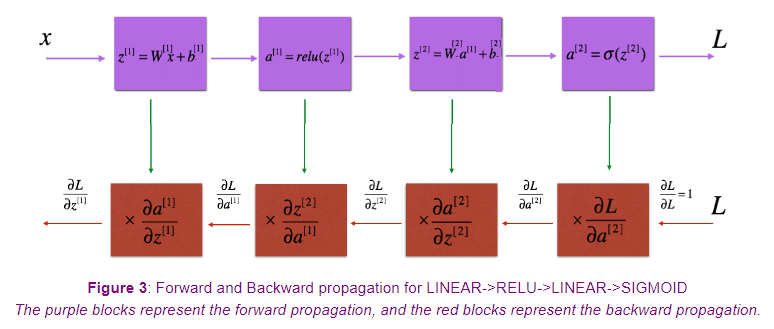
Now, similarly to forward propagation, you’re going to build the backward propagation in three steps:

1. LINEAR backward
2. LINEAR -> ACTIVATION backward where ACTIVATION computes the derivative of either the ReLU or sigmoid activation
3. [LINEAR -> RELU] $\times$ (L-1) -> LINEAR -> SIGMOID backward (whole model)

For the next exercise, you will need to remember that:

• b is a matrix(np.ndarray) with 1 column and n rows, i.e: b = [[1.0], [2.0]] (remember that b is a constant)
• np.sum performs a sum over the elements of a ndarray
• axis=1 or axis=0 specify if the sum is carried out by rows or by columns respectively
• keepdims specifies if the original dimensions of the matrix must be kept.
• Look at the following example to clarify:

A = np.array([[1, 2], [3, 4]])

print('axis=1 and keepdims=True')
print(np.sum(A, axis=1, keepdims=True))
print('axis=1 and keepdims=False')
print(np.sum(A, axis=1, keepdims=False))
print('axis=0 and keepdims=True')
print(np.sum(A, axis=0, keepdims=True))
print('axis=0 and keepdims=False')
print(np.sum(A, axis=0, keepdims=False))

Output

axis=1 and keepdims=True
[[3]
 [7]]
axis=1 and keepdims=False
[3 7]
axis=0 and keepdims=True
[[4 6]]
axis=0 and keepdims=False
[4 6]

6.1 - Linear Backward

For layer $l$, the linear part is: $Z^{[l]}=W^{[l]}{A}^{[l-1]}+b^{[l]}$ (followed by an activation).

Suppose you have already calculated the derivative $d{Z}^{[l]}=\frac{\partial \mathcal{L}}{\partial Z^{[l]}}$. You want to get $(d{W}^{[l]},d{b}^{[l]},d{A}^{[l-1]})$.

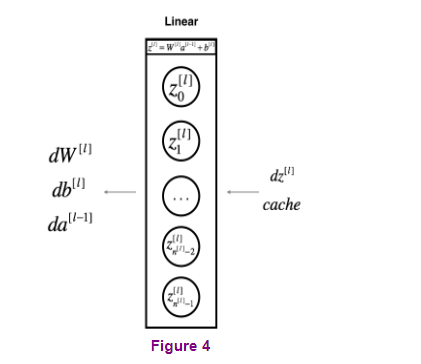
The three outputs $(d{W}^{[l]},d{b}^{[l]},d{A}^{[l-1]})$ are computed using the input $d{Z}^{[l]}$.

Here are the formulas you need:
$$d{W}^{[l]}=\frac{\partial \mathcal{J}}{\partial W^{[l]}}=\frac{1}{m}d{Z}^{[l]}{A}^{[l-1]T}\text{\hspace{1em}(8)}$$
$$d{b}^{[l]}=\frac{\partial \mathcal{J}}{\partial b^{[l]}}=\frac{1}{m}\sum _{i=1}^{m}d{Z}^{[l](i)}\text{\hspace{1em}(9)}$$
$$d{A}^{[l-1]}=\frac{\partial \mathcal{L}}{\partial A^{[l-1]}}=W^{[l]T}d{Z}^{[l]}\text{\hspace{1em}(10)}$$

$A^{[l-1]T}$ is the transpose of $A^{[l-1]}$.

Exercise 7 - linear_backward

Use the 3 formulas above to implement linear_backward().

Hint:

• In numpy you can get the transpose of an ndarray A using A.T or A.transpose()

# GRADED FUNCTION: linear_backward

def linear_backward(dZ, cache):
    """
    Implement the linear portion of backward propagation for a single layer (layer l)

    Arguments:
    dZ -- Gradient of the cost with respect to the linear output (of current layer l)
    cache -- tuple of values (A_prev, W, b) coming from the forward propagation in the current layer

    Returns:
    dA_prev -- Gradient of the cost with respect to the activation (of the previous layer l-1), same shape as A_prev
    dW -- Gradient of the cost with respect to W (current layer l), same shape as W
    db -- Gradient of the cost with respect to b (current layer l), same shape as b
    """
    A_prev, W, b = cache
    m = A_prev.shape[1]

    ### START CODE HERE ### (≈ 3 lines of code)
    # dW = ...
    # db = ... sum by the rows of dZ with keepdims=True
    # dA_prev = ...
    # YOUR CODE STARTS HERE
    dW = 1 / m * np.dot(dZ, A_prev.T)
    db = 1 / m * np.sum(dZ, axis=1, keepdims=True)
    dA_prev = np.dot(W.T, dZ)
    
    # YOUR CODE ENDS HERE
    
    return dA_prev, dW, db

t_dZ, t_linear_cache = linear_backward_test_case()
t_dA_prev, t_dW, t_db = linear_backward(t_dZ, t_linear_cache)

print("dA_prev: " + str(t_dA_prev))
print("dW: " + str(t_dW))
print("db: " + str(t_db))

linear_backward_test(linear_backward)

Output

dA_prev: [[-1.15171336  0.06718465 -0.3204696   2.09812712]
 [ 0.60345879 -3.72508701  5.81700741 -3.84326836]
 [-0.4319552  -1.30987417  1.72354705  0.05070578]
 [-0.38981415  0.60811244 -1.25938424  1.47191593]
 [-2.52214926  2.67882552 -0.67947465  1.48119548]]
dW: [[ 0.07313866 -0.0976715  -0.87585828  0.73763362  0.00785716]
 [ 0.85508818  0.37530413 -0.59912655  0.71278189 -0.58931808]
 [ 0.97913304 -0.24376494 -0.08839671  0.55151192 -0.10290907]]
db: [[-0.14713786]
 [-0.11313155]
 [-0.13209101]]
 All tests passed.

Expected Output:

dA_prev: [[-1.15171336  0.06718465 -0.3204696   2.09812712]
 [ 0.60345879 -3.72508701  5.81700741 -3.84326836]
 [-0.4319552  -1.30987417  1.72354705  0.05070578]
 [-0.38981415  0.60811244 -1.25938424  1.47191593]
 [-2.52214926  2.67882552 -0.67947465  1.48119548]]
dW: [[ 0.07313866 -0.0976715  -0.87585828  0.73763362  0.00785716]
 [ 0.85508818  0.37530413 -0.59912655  0.71278189 -0.58931808]
 [ 0.97913304 -0.24376494 -0.08839671  0.55151192 -0.10290907]]
db: [[-0.14713786]
 [-0.11313155]
 [-0.13209101]]

6.2 - Linear-Activation Backward

Next, you will create a function that merges the two helper functions: linear_backward and the backward step for the activation linear_activation_backward.

To help you implement linear_activation_backward, two backward functions have been provided:

• sigmoid_backward: Implements the backward propagation for SIGMOID unit. You can call it as follows:

dZ = sigmoid_backward(dA, activation_cache)

• relu_backward: Implements the backward propagation for RELU unit. You can call it as follows:

dZ = relu_backward(dA, activation_cache)

If $g(.)$ is the activation function,
sigmoid_backward and relu_backward compute $$d{Z}^{[l]}=d{A}^{[l]}\ast g^{\prime }(Z^{[l]}).\text{\hspace{1em}(11)}$$

Exercise 8 - linear_activation_backward

Implement the backpropagation for the LINEAR->ACTIVATION layer.

# GRADED FUNCTION: linear_activation_backward

def linear_activation_backward(dA, cache, activation):
    """
    Implement the backward propagation for the LINEAR->ACTIVATION layer.
    
    Arguments:
    dA -- post-activation gradient for current layer l 
    cache -- tuple of values (linear_cache, activation_cache) we store for computing backward propagation efficiently
    activation -- the activation to be used in this layer, stored as a text string: "sigmoid" or "relu"
    
    Returns:
    dA_prev -- Gradient of the cost with respect to the activation (of the previous layer l-1), same shape as A_prev
    dW -- Gradient of the cost with respect to W (current layer l), same shape as W
    db -- Gradient of the cost with respect to b (current layer l), same shape as b
    """
    linear_cache, activation_cache = cache
    
    if activation == "relu":
        #(≈ 2 lines of code)
        # dZ =  ...
        # dA_prev, dW, db =  ...
        # YOUR CODE STARTS HERE
        dZ = relu_backward(dA, activation_cache)
        dA_prev, dW, db = linear_backward(dZ, linear_cache)
        
        # YOUR CODE ENDS HERE
        
    elif activation == "sigmoid":
        #(≈ 2 lines of code)
        # dZ =  ...
        # dA_prev, dW, db =  ...
        # YOUR CODE STARTS HERE
        dZ = sigmoid_backward(dA, activation_cache)
        dA_prev, dW, db = linear_backward(dZ, linear_cache)
        
        # YOUR CODE ENDS HERE
    
    return dA_prev, dW, db

t_dAL, t_linear_activation_cache = linear_activation_backward_test_case()

t_dA_prev, t_dW, t_db = linear_activation_backward(t_dAL, t_linear_activation_cache, activation = "sigmoid")
print("With sigmoid: dA_prev = " + str(t_dA_prev))
print("With sigmoid: dW = " + str(t_dW))
print("With sigmoid: db = " + str(t_db))

t_dA_prev, t_dW, t_db = linear_activation_backward(t_dAL, t_linear_activation_cache, activation = "relu")
print("With relu: dA_prev = " + str(t_dA_prev))
print("With relu: dW = " + str(t_dW))
print("With relu: db = " + str(t_db))

linear_activation_backward_test(linear_activation_backward)

Output

With sigmoid: dA_prev = [[ 0.11017994  0.01105339]
 [ 0.09466817  0.00949723]
 [-0.05743092 -0.00576154]]
With sigmoid: dW = [[ 0.10266786  0.09778551 -0.01968084]]
With sigmoid: db = [[-0.05729622]]
With relu: dA_prev = [[ 0.44090989  0.        ]
 [ 0.37883606  0.        ]
 [-0.2298228   0.        ]]
With relu: dW = [[ 0.44513824  0.37371418 -0.10478989]]
With relu: db = [[-0.20837892]]
 All tests passed.

Expected output:

With sigmoid: dA_prev = [[ 0.11017994  0.01105339]
 [ 0.09466817  0.00949723]
 [-0.05743092 -0.00576154]]
With sigmoid: dW = [[ 0.10266786  0.09778551 -0.01968084]]
With sigmoid: db = [[-0.05729622]]
With relu: dA_prev = [[ 0.44090989  0.        ]
 [ 0.37883606  0.        ]
 [-0.2298228   0.        ]]
With relu: dW = [[ 0.44513824  0.37371418 -0.10478989]]
With relu: db = [[-0.20837892]]

6.3 - L-Model Backward

Now you will implement the backward function for the whole network!

Recall that when you implemented the L_model_forward function, at each iteration, you stored a cache which contains (X,W,b, and z). In the back propagation module, you’ll use those variables to compute the gradients. Therefore, in the L_model_backward function, you’ll iterate through all the hidden layers backward, starting from layer $L$. On each step, you will use the cached values for layer $l$ to backpropagate through layer $l$. Figure 5 below shows the backward pass.

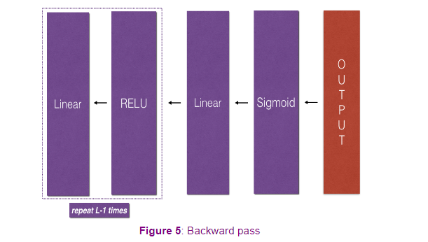
Initializing backpropagation:

To backpropagate through this network, you know that the output is:
$A^{[L]}=\sigma (Z^{[L]})$. Your code thus needs to compute dAL $=\frac{\partial \mathcal{L}}{\partial A^{[L]}}$.
To do so, use this formula (derived using calculus which, again, you don’t need in-depth knowledge of!):

dAL = - (np.divide(Y, AL) - np.divide(1 - Y, 1 - AL)) # derivative of cost with respect to AL

You can then use this post-activation gradient dAL to keep going backward. As seen in Figure 5, you can now feed in dAL into the LINEAR->SIGMOID backward function you implemented (which will use the cached values stored by the L_model_forward function).

After that, you will have to use a for loop to iterate through all the other layers using the LINEAR->RELU backward function. You should store each dA, dW, and db in the grads dictionary. To do so, use this formula :

$$grads["dW"+str(l)]=d{W}^{[l]}\text{\hspace{1em}(15)}$$

For example, for $l=3$ this would store $d{W}^{[l]}$ in grads["dW3"].

Exercise 9 - L_model_backward

Implement backpropagation for the [LINEAR->RELU] $\times$ (L-1) -> LINEAR -> SIGMOID model.

# GRADED FUNCTION: L_model_backward

def L_model_backward(AL, Y, caches):
    """
    Implement the backward propagation for the [LINEAR->RELU] * (L-1) -> LINEAR -> SIGMOID group
    
    Arguments:
    AL -- probability vector, output of the forward propagation (L_model_forward())
    Y -- true "label" vector (containing 0 if non-cat, 1 if cat)
    caches -- list of caches containing:
                every cache of linear_activation_forward() with "relu" (it's caches[l], for l in range(L-1) i.e l = 0...L-2)
                the cache of linear_activation_forward() with "sigmoid" (it's caches[L-1])
    
    Returns:
    grads -- A dictionary with the gradients
             grads["dA" + str(l)] = ... 
             grads["dW" + str(l)] = ...
             grads["db" + str(l)] = ... 
    """
    grads = {}
    L = len(caches) # the number of layers
    m = AL.shape[1]
    Y = Y.reshape(AL.shape) # after this line, Y is the same shape as AL
    
    # Initializing the backpropagation
    #(1 line of code)
    # dAL = ...
    # YOUR CODE STARTS HERE
    dAL = - (np.divide(Y, AL) - np.divide(1 - Y, 1 - AL))
    
    # YOUR CODE ENDS HERE
    
    # Lth layer (SIGMOID -> LINEAR) gradients. Inputs: "dAL, current_cache". Outputs: "grads["dAL-1"], grads["dWL"], grads["dbL"]
    #(approx. 5 lines)
    # current_cache = ...
    # dA_prev_temp, dW_temp, db_temp = ...
    # grads["dA" + str(L-1)] = ...
    # grads["dW" + str(L)] = ...
    # grads["db" + str(L)] = ...
    # YOUR CODE STARTS HERE
    current_cache = caches[L-1]
    dA_prev_temp, dW_temp, db_temp = linear_activation_backward(dAL, current_cache, activation="sigmoid")
    grads["dA" + str(L-1)] = dA_prev_temp
    grads["dW" + str(L)] = dW_temp
    grads["db" + str(L)] = db_temp
    
    # YOUR CODE ENDS HERE
    
    # Loop from l=L-2 to l=0
    for l in reversed(range(L-1)):
        # lth layer: (RELU -> LINEAR) gradients.
        # Inputs: "grads["dA" + str(l + 1)], current_cache". Outputs: "grads["dA" + str(l)] , grads["dW" + str(l + 1)] , grads["db" + str(l + 1)] 
        #(approx. 5 lines)
        # current_cache = ...
        # dA_prev_temp, dW_temp, db_temp = ...
        # grads["dA" + str(l)] = ...
        # grads["dW" + str(l + 1)] = ...
        # grads["db" + str(l + 1)] = ...
        # YOUR CODE STARTS HERE
        current_cache = caches[l]
        dA_prev_temp, dW_temp, db_temp = linear_activation_backward(grads["dA" + str(l + 1)], current_cache, activation="relu")
        grads["dA" + str(l)] = dA_prev_temp
        grads["dW" + str(l + 1)] = dW_temp
        grads["db" + str(l + 1)] = db_temp
        
        # YOUR CODE ENDS HERE

    return grads

t_AL, t_Y_assess, t_caches = L_model_backward_test_case()
grads = L_model_backward(t_AL, t_Y_assess, t_caches)

print("dA0 = " + str(grads['dA0']))
print("dA1 = " + str(grads['dA1']))
print("dW1 = " + str(grads['dW1']))
print("dW2 = " + str(grads['dW2']))
print("db1 = " + str(grads['db1']))
print("db2 = " + str(grads['db2']))

L_model_backward_test(L_model_backward)

Output

dA0 = [[ 0.          0.52257901]
 [ 0.         -0.3269206 ]
 [ 0.         -0.32070404]
 [ 0.         -0.74079187]]
dA1 = [[ 0.12913162 -0.44014127]
 [-0.14175655  0.48317296]
 [ 0.01663708 -0.05670698]]
dW1 = [[0.41010002 0.07807203 0.13798444 0.10502167]
 [0.         0.         0.         0.        ]
 [0.05283652 0.01005865 0.01777766 0.0135308 ]]
dW2 = [[-0.39202432 -0.13325855 -0.04601089]]
db1 = [[-0.22007063]
 [ 0.        ]
 [-0.02835349]]
db2 = [[0.15187861]]
 All tests passed.

Expected output:

dA0 = [[ 0.          0.52257901]
 [ 0.         -0.3269206 ]
 [ 0.         -0.32070404]
 [ 0.         -0.74079187]]
dA1 = [[ 0.12913162 -0.44014127]
 [-0.14175655  0.48317296]
 [ 0.01663708 -0.05670698]]
dW1 = [[0.41010002 0.07807203 0.13798444 0.10502167]
 [0.         0.         0.         0.        ]
 [0.05283652 0.01005865 0.01777766 0.0135308 ]]
dW2 = [[-0.39202432 -0.13325855 -0.04601089]]
db1 = [[-0.22007063]
 [ 0.        ]
 [-0.02835349]]
db2 = [[0.15187861]]

6.4 - Update Parameters

In this section, you’ll update the parameters of the model, using gradient descent:

$$W^{[l]}=W^{[l]}-\alpha d{W}^{[l]}\text{\hspace{1em}(16)}$$
$$b^{[l]}=b^{[l]}-\alpha d{b}^{[l]}\text{\hspace{1em}(17)}$$

where $\alpha$ is the learning rate.

After computing the updated parameters, store them in the parameters dictionary.

Exercise 10 - update_parameters

Implement update_parameters() to update your parameters using gradient descent.

Instructions:
Update parameters using gradient descent on every $W^{[l]}$ and $b^{[l]}$ for $l=1,2,...,L$.

# GRADED FUNCTION: update_parameters

def update_parameters(params, grads, learning_rate):
    """
    Update parameters using gradient descent
    
    Arguments:
    params -- python dictionary containing your parameters 
    grads -- python dictionary containing your gradients, output of L_model_backward
    
    Returns:
    parameters -- python dictionary containing your updated parameters 
                  parameters["W" + str(l)] = ... 
                  parameters["b" + str(l)] = ...
    """
    parameters = copy.deepcopy(params)
    L = len(parameters) // 2 # number of layers in the neural network

    # Update rule for each parameter. Use a for loop.
    #(≈ 2 lines of code)
    for l in range(L):
        # parameters["W" + str(l+1)] = ...
        # parameters["b" + str(l+1)] = ...
        # YOUR CODE STARTS HERE
        parameters["W" + str(l + 1)] -= learning_rate * grads["dW" + str(l + 1)]
        parameters["b" + str(l + 1)] -= learning_rate * grads["db" + str(l + 1)]

        
        # YOUR CODE ENDS HERE
    return parameters

t_parameters, grads = update_parameters_test_case()
t_parameters = update_parameters(t_parameters, grads, 0.1)

print ("W1 = "+ str(t_parameters["W1"]))
print ("b1 = "+ str(t_parameters["b1"]))
print ("W2 = "+ str(t_parameters["W2"]))
print ("b2 = "+ str(t_parameters["b2"]))

update_parameters_test(update_parameters)

Output

W1 = [[-0.59562069 -0.09991781 -2.14584584  1.82662008]
 [-1.76569676 -0.80627147  0.51115557 -1.18258802]
 [-1.0535704  -0.86128581  0.68284052  2.20374577]]
b1 = [[-0.04659241]
 [-1.28888275]
 [ 0.53405496]]
W2 = [[-0.55569196  0.0354055   1.32964895]]
b2 = [[-0.84610769]]
 All tests passed.

Expected output:

W1 = [[-0.59562069 -0.09991781 -2.14584584  1.82662008]
 [-1.76569676 -0.80627147  0.51115557 -1.18258802]
 [-1.0535704  -0.86128581  0.68284052  2.20374577]]
b1 = [[-0.04659241]
 [-1.28888275]
 [ 0.53405496]]
W2 = [[-0.55569196  0.0354055   1.32964895]]
b2 = [[-0.84610769]]

Congratulations!

You’ve just implemented all the functions required for building a deep neural network, including:

• Using non-linear units improve your model
• Building a deeper neural network (with more than 1 hidden layer)
• Implementing an easy-to-use neural network class

This was indeed a long assignment, but the next part of the assignment is easier. 😉

In the next assignment, you’ll be putting all these together to build two models:

• A two-layer neural network
• An L-layer neural network

You will in fact use these models to classify cat vs non-cat images! (Meow!) Great work and see you next time.

Grades

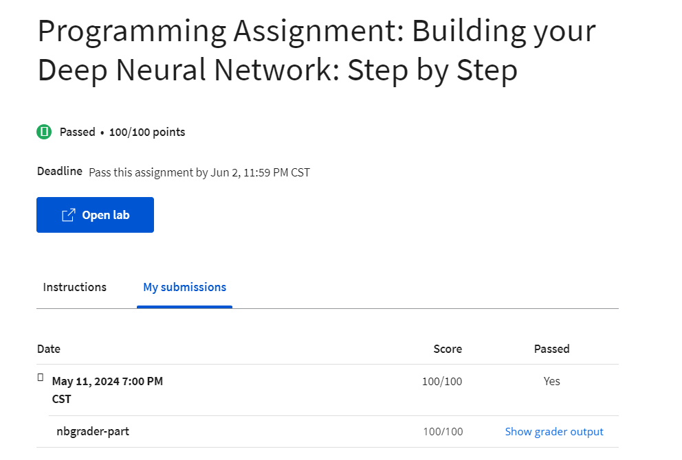
Programming Assignment: Deep Neural Network - Application

Deep Neural Network for Image Classification: Application

By the time you complete this notebook, you will have finished the last programming assignment of Week 4, and also the last programming assignment of Course 1! Go you!

To build your cat/not-a-cat classifier, you’ll use the functions from the previous assignment to build a deep network. Hopefully, you’ll see an improvement in accuracy over your previous logistic regression implementation.

After this assignment you will be able to:

• Build and train a deep L-layer neural network, and apply it to supervised learning

Let’s get started!

Important Note on Submission to the AutoGrader

Before submitting your assignment to the AutoGrader, please make sure you are not doing the following:

1. You have not added any extra print statement(s) in the assignment.
2. You have not added any extra code cell(s) in the assignment.
3. You have not changed any of the function parameters.
4. You are not using any global variables inside your graded exercises. Unless specifically instructed to do so, please refrain from it and use the local variables instead.
5. You are not changing the assignment code where it is not required, like creating extra variables.

If you do any of the following, you will get something like, Grader Error: Grader feedback not found (or similarly unexpected) error upon submitting your assignment. Before asking for help/debugging the errors in your assignment, check for these first. If this is the case, and you don’t remember the changes you have made, you can get a fresh copy of the assignment by following these instructions.

1 - Packages

Begin by importing all the packages you’ll need during this assignment.

• numpy is the fundamental package for scientific computing with Python.
• matplotlib is a library to plot graphs in Python.
• h5py is a common package to interact with a dataset that is stored on an H5 file.
• PIL and scipy are used here to test your model with your own picture at the end.
• dnn_app_utils provides the functions implemented in the “Building your Deep Neural Network: Step by Step” assignment to this notebook.
• np.random.seed(1) is used to keep all the random function calls consistent. It helps grade your work - so please don’t change it!

import time
import numpy as np
import h5py
import matplotlib.pyplot as plt
import scipy
from PIL import Image
from scipy import ndimage
from dnn_app_utils_v3 import *
from public_tests import *

%matplotlib inline
plt.rcParams['figure.figsize'] = (5.0, 4.0) # set default size of plots
plt.rcParams['image.interpolation'] = 'nearest'
plt.rcParams['image.cmap'] = 'gray'

%load_ext autoreload
%autoreload 2

np.random.seed(1)

2 - Load and Process the Dataset

You’ll be using the same “Cat vs non-Cat” dataset as in “Logistic Regression as a Neural Network” (Assignment 2). The model you built back then had 70% test accuracy on classifying cat vs non-cat images. Hopefully, your new model will perform even better!

Problem Statement: You are given a dataset (“data.h5”) containing:
- a training set of m_train images labelled as cat (1) or non-cat (0)
- a test set of m_test images labelled as cat and non-cat
- each image is of shape (num_px, num_px, 3) where 3 is for the 3 channels (RGB).

Let’s get more familiar with the dataset. Load the data by running the cell below.

train_x_orig, train_y, test_x_orig, test_y, classes = load_data()

The following code will show you an image in the dataset. Feel free to change the index and re-run the cell multiple times to check out other images.

# Example of a picture
index = 10
plt.imshow(train_x_orig[index])
print ("y = " + str(train_y[0,index]) + ". It's a " + classes[train_y[0,index]].decode("utf-8") +  " picture.")

Output

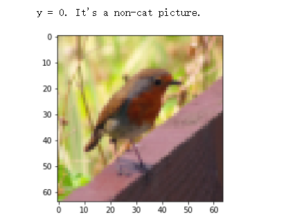
# Explore your dataset 
m_train = train_x_orig.shape[0]
num_px = train_x_orig.shape[1]
m_test = test_x_orig.shape[0]

print ("Number of training examples: " + str(m_train))
print ("Number of testing examples: " + str(m_test))
print ("Each image is of size: (" + str(num_px) + ", " + str(num_px) + ", 3)")
print ("train_x_orig shape: " + str(train_x_orig.shape))
print ("train_y shape: " + str(train_y.shape))
print ("test_x_orig shape: " + str(test_x_orig.shape))
print ("test_y shape: " + str(test_y.shape))

Output

Number of training examples: 209
Number of testing examples: 50
Each image is of size: (64, 64, 3)
train_x_orig shape: (209, 64, 64, 3)
train_y shape: (1, 209)
test_x_orig shape: (50, 64, 64, 3)
test_y shape: (1, 50)

As usual, you reshape and standardize the images before feeding them to the network. The code is given in the cell below.

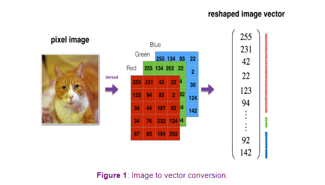
# Reshape the training and test examples 
train_x_flatten = train_x_orig.reshape(train_x_orig.shape[0], -1).T   # The "-1" makes reshape flatten the remaining dimensions
test_x_flatten = test_x_orig.reshape(test_x_orig.shape[0], -1).T

# Standardize data to have feature values between 0 and 1.
train_x = train_x_flatten/255.
test_x = test_x_flatten/255.

print ("train_x's shape: " + str(train_x.shape))
print ("test_x's shape: " + str(test_x.shape))

Output

train_x's shape: (12288, 209)
test_x's shape: (12288, 50)

Note:
$12,288$ equals $64\times 64\times 3$, which is the size of one reshaped image vector.

3 - Model Architecture

3.1 - 2-layer Neural Network

Now that you’re familiar with the dataset, it’s time to build a deep neural network to distinguish cat images from non-cat images!

You’re going to build two different models:

• A 2-layer neural network
• An L-layer deep neural network

Then, you’ll compare the performance of these models, and try out some different values for $L$.

Let’s look at the two architectures:

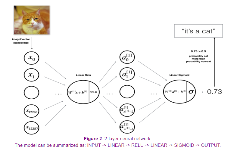
Detailed Architecture of Figure 2:

• The input is a (64,64,3) image which is flattened to a vector of size $(12288,1)$.
• The corresponding vector: $[x_0,x_1,...,x_{12287}{]}^T$ is then multiplied by the weight matrix $W^{[1]}$ of size $(n^{[1]},12288)$.
• Then, add a bias term and take its relu to get the following vector: $[a_0^{[1]},a_1^{[1]},...,a_{n^{[1]}-1}^{[1]}{]}^T$.
• Multiply the resulting vector by $W^{[2]}$ and add the intercept (bias).
• Finally, take the sigmoid of the result. If it’s greater than 0.5, classify it as a cat.

3.2 - L-layer Deep Neural Network

It’s pretty difficult to represent an L-layer deep neural network using the above representation. However, here is a simplified network representation:

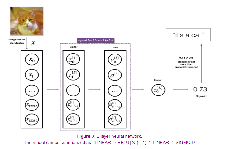
Detailed Architecture of Figure 3:

• The input is a (64,64,3) image which is flattened to a vector of size (12288,1).
• The corresponding vector: $[x_0,x_1,...,x_{12287}{]}^T$ is then multiplied by the weight matrix $W^{[1]}$ and then you add the intercept $b^{[1]}$. The result is called the linear unit.
• Next, take the relu of the linear unit. This process could be repeated several times for each $(W^{[l]},b^{[l]})$ depending on the model architecture.
• Finally, take the sigmoid of the final linear unit. If it is greater than 0.5, classify it as a cat.

3.3 - General Methodology

As usual, you’ll follow the Deep Learning methodology to build the model:

1. Initialize parameters / Define hyperparameters
2. Loop for num_iterations:
   a. Forward propagation
   b. Compute cost function
   c. Backward propagation
   d. Update parameters (using parameters, and grads from backprop)
3. Use trained parameters to predict labels

Now go ahead and implement those two models!

4 - Two-layer Neural Network

Exercise 1 - two_layer_model

Use the helper functions you have implemented in the previous assignment to build a 2-layer neural network with the following structure: LINEAR -> RELU -> LINEAR -> SIGMOID. The functions and their inputs are:

def initialize_parameters(n_x, n_h, n_y):
    ...
    return parameters 
def linear_activation_forward(A_prev, W, b, activation):
    ...
    return A, cache
def compute_cost(AL, Y):
    ...
    return cost
def linear_activation_backward(dA, cache, activation):
    ...
    return dA_prev, dW, db
def update_parameters(parameters, grads, learning_rate):
    ...
    return parameters

### CONSTANTS DEFINING THE MODEL ####
n_x = 12288     # num_px * num_px * 3
n_h = 7
n_y = 1
layers_dims = (n_x, n_h, n_y)
learning_rate = 0.0075

# GRADED FUNCTION: two_layer_model

def two_layer_model(X, Y, layers_dims, learning_rate = 0.0075, num_iterations = 3000, print_cost=False):
    """
    Implements a two-layer neural network: LINEAR->RELU->LINEAR->SIGMOID.
    
    Arguments:
    X -- input data, of shape (n_x, number of examples)
    Y -- true "label" vector (containing 1 if cat, 0 if non-cat), of shape (1, number of examples)
    layers_dims -- dimensions of the layers (n_x, n_h, n_y)
    num_iterations -- number of iterations of the optimization loop
    learning_rate -- learning rate of the gradient descent update rule
    print_cost -- If set to True, this will print the cost every 100 iterations 
    
    Returns:
    parameters -- a dictionary containing W1, W2, b1, and b2
    """
    
    np.random.seed(1)
    grads = {}
    costs = []                              # to keep track of the cost
    m = X.shape[1]                           # number of examples
    (n_x, n_h, n_y) = layers_dims
    
    # Initialize parameters dictionary, by calling one of the functions you'd previously implemented
    #(≈ 1 line of code)
    # parameters = ...
    # YOUR CODE STARTS HERE
    parameters = initialize_parameters(n_x, n_h, n_y)
    
    # YOUR CODE ENDS HERE
    
    # Get W1, b1, W2 and b2 from the dictionary parameters.
    W1 = parameters["W1"]
    b1 = parameters["b1"]
    W2 = parameters["W2"]
    b2 = parameters["b2"]
    
    # Loop (gradient descent)

    for i in range(0, num_iterations):

        # Forward propagation: LINEAR -> RELU -> LINEAR -> SIGMOID. Inputs: "X, W1, b1, W2, b2". Output: "A1, cache1, A2, cache2".
        #(≈ 2 lines of code)
        # A1, cache1 = ...
        # A2, cache2 = ...
        # YOUR CODE STARTS HERE
        A1, cache1 = linear_activation_forward(X, W1, b1, activation="relu")
        A2, cache2 = linear_activation_forward(A1, W2, b2, activation="sigmoid")
        
        # YOUR CODE ENDS HERE
        
        # Compute cost
        #(≈ 1 line of code)
        # cost = ...
        # YOUR CODE STARTS HERE
        cost = compute_cost(A2, Y)
        
        # YOUR CODE ENDS HERE
        
        # Initializing backward propagation
        dA2 = - (np.divide(Y, A2) - np.divide(1 - Y, 1 - A2))
        
        # Backward propagation. Inputs: "dA2, cache2, cache1". Outputs: "dA1, dW2, db2; also dA0 (not used), dW1, db1".
        #(≈ 2 lines of code)
        # dA1, dW2, db2 = ...
        # dA0, dW1, db1 = ...
        # YOUR CODE STARTS HERE
        dA1, dW2, db2 = linear_activation_backward(dA2, cache2, activation="sigmoid")
        dA0, dW1, db1 = linear_activation_backward(dA1, cache1, activation="relu")
        
        # YOUR CODE ENDS HERE
        
        # Set grads['dWl'] to dW1, grads['db1'] to db1, grads['dW2'] to dW2, grads['db2'] to db2
        grads['dW1'] = dW1
        grads['db1'] = db1
        grads['dW2'] = dW2
        grads['db2'] = db2
        
        # Update parameters.
        #(approx. 1 line of code)
        # parameters = ...
        # YOUR CODE STARTS HERE
        parameters = update_parameters(parameters, grads, learning_rate)
        
        # YOUR CODE ENDS HERE

        # Retrieve W1, b1, W2, b2 from parameters
        W1 = parameters["W1"]
        b1 = parameters["b1"]
        W2 = parameters["W2"]
        b2 = parameters["b2"]
        
        # Print the cost every 100 iterations
        if print_cost and i % 100 == 0 or i == num_iterations - 1:
            print("Cost after iteration {}: {}".format(i, np.squeeze(cost)))
        if i % 100 == 0 or i == num_iterations:
            costs.append(cost)

    return parameters, costs

def plot_costs(costs, learning_rate=0.0075):
    plt.plot(np.squeeze(costs))
    plt.ylabel('cost')
    plt.xlabel('iterations (per hundreds)')
    plt.title("Learning rate =" + str(learning_rate))
    plt.show()

parameters, costs = two_layer_model(train_x, train_y, layers_dims = (n_x, n_h, n_y), num_iterations = 2, print_cost=False)

print("Cost after first iteration: " + str(costs[0]))

two_layer_model_test(two_layer_model)

Output

Cost after iteration 1: 0.6926114346158595
Cost after first iteration: 0.693049735659989
Cost after iteration 1: 0.6915746967050506
Cost after iteration 1: 0.6915746967050506
Cost after iteration 1: 0.6915746967050506
Cost after iteration 2: 0.6524135179683452
 All tests passed.

Expected output:

cost after iteration 1 must be around 0.69

4.1 - Train the model

If your code passed the previous cell, run the cell below to train your parameters.

• The cost should decrease on every iteration.

• It may take up to 5 minutes to run 2500 iterations.

parameters, costs = two_layer_model(train_x, train_y, layers_dims = (n_x, n_h, n_y), num_iterations = 2500, print_cost=True)
plot_costs(costs, learning_rate)

Output

Cost after iteration 0: 0.693049735659989
Cost after iteration 100: 0.6464320953428849
Cost after iteration 200: 0.6325140647912677
Cost after iteration 300: 0.6015024920354665
Cost after iteration 400: 0.5601966311605747
Cost after iteration 500: 0.5158304772764729
Cost after iteration 600: 0.4754901313943325
Cost after iteration 700: 0.43391631512257495
Cost after iteration 800: 0.4007977536203886
Cost after iteration 900: 0.3580705011323798
Cost after iteration 1000: 0.3394281538366413
Cost after iteration 1100: 0.30527536361962654
Cost after iteration 1200: 0.2749137728213015
Cost after iteration 1300: 0.2468176821061484
Cost after iteration 1400: 0.19850735037466102
Cost after iteration 1500: 0.17448318112556638
Cost after iteration 1600: 0.1708076297809692
Cost after iteration 1700: 0.11306524562164715
Cost after iteration 1800: 0.09629426845937156
Cost after iteration 1900: 0.0834261795972687
Cost after iteration 2000: 0.07439078704319085
Cost after iteration 2100: 0.06630748132267933
Cost after iteration 2200: 0.05919329501038172
Cost after iteration 2300: 0.053361403485605606
Cost after iteration 2400: 0.04855478562877019
Cost after iteration 2499: 0.04421498215868956

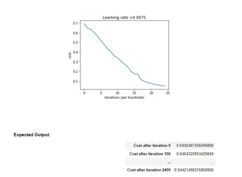
Nice! You successfully trained the model. Good thing you built a vectorized implementation! Otherwise it might have taken 10 times longer to train this.

Now, you can use the trained parameters to classify images from the dataset. To see your predictions on the training and test sets, run the cell below.

predictions_train = predict(train_x, train_y, parameters)

Output

Accuracy: 0.9999999999999998

Expected Output:

Accuracy

0.9999999999999998

predictions_test = predict(test_x, test_y, parameters)

Output

Accuracy: 0.72

Expected Output:

Accuracy

0.72

Congratulations! It seems that your 2-layer neural network has better performance (72%) than the logistic regression implementation (70%, assignment week 2). Let’s see if you can do even better with an $L$-layer model.

Note: You may notice that running the model on fewer iterations (say 1500) gives better accuracy on the test set. This is called “early stopping” and you’ll hear more about it in the next course. Early stopping is a way to prevent overfitting.

5 - L-layer Neural Network

Exercise 2 - L_layer_model

Use the helper functions you implemented previously to build an $L$-layer neural network with the following structure: [LINEAR -> RELU]$\times$(L-1) -> LINEAR -> SIGMOID. The functions and their inputs are:

def initialize_parameters_deep(layers_dims):
    ...
    return parameters 
def L_model_forward(X, parameters):
    ...
    return AL, caches
def compute_cost(AL, Y):
    ...
    return cost
def L_model_backward(AL, Y, caches):
    ...
    return grads
def update_parameters(parameters, grads, learning_rate):
    ...
    return parameters

### CONSTANTS ###
layers_dims = [12288, 20, 7, 5, 1] #  4-layer model

# GRADED FUNCTION: L_layer_model

def L_layer_model(X, Y, layers_dims, learning_rate = 0.0075, num_iterations = 3000, print_cost=False):
    """
    Implements a L-layer neural network: [LINEAR->RELU]*(L-1)->LINEAR->SIGMOID.
    
    Arguments:
    X -- input data, of shape (n_x, number of examples)
    Y -- true "label" vector (containing 1 if cat, 0 if non-cat), of shape (1, number of examples)
    layers_dims -- list containing the input size and each layer size, of length (number of layers + 1).
    learning_rate -- learning rate of the gradient descent update rule
    num_iterations -- number of iterations of the optimization loop
    print_cost -- if True, it prints the cost every 100 steps
    
    Returns:
    parameters -- parameters learnt by the model. They can then be used to predict.
    """

    np.random.seed(1)
    costs = []                         # keep track of cost
    
    # Parameters initialization.
    #(≈ 1 line of code)
    # parameters = ...
    # YOUR CODE STARTS HERE
    parameters = initialize_parameters_deep(layers_dims)
    
    # YOUR CODE ENDS HERE
    
    # Loop (gradient descent)
    for i in range(0, num_iterations):

        # Forward propagation: [LINEAR -> RELU]*(L-1) -> LINEAR -> SIGMOID.
        #(≈ 1 line of code)
        # AL, caches = ...
        # YOUR CODE STARTS HERE
        AL, caches = L_model_forward(X, parameters)
        
        # YOUR CODE ENDS HERE
        
        # Compute cost.
        #(≈ 1 line of code)
        # cost = ...
        # YOUR CODE STARTS HERE
        cost = compute_cost(AL, Y)
        
        # YOUR CODE ENDS HERE
    
        # Backward propagation.
        #(≈ 1 line of code)
        # grads = ...    
        # YOUR CODE STARTS HERE
        grads = L_model_backward(AL, Y, caches)
        
        # YOUR CODE ENDS HERE
 
        # Update parameters.
        #(≈ 1 line of code)
        # parameters = ...
        # YOUR CODE STARTS HERE
        parameters = update_parameters(parameters, grads, learning_rate)
        
        # YOUR CODE ENDS HERE
                
        # Print the cost every 100 iterations
        if print_cost and i % 100 == 0 or i == num_iterations - 1:
            print("Cost after iteration {}: {}".format(i, np.squeeze(cost)))
        if i % 100 == 0 or i == num_iterations:
            costs.append(cost)
    
    return parameters, costs

parameters, costs = L_layer_model(train_x, train_y, layers_dims, num_iterations = 1, print_cost = False)

print("Cost after first iteration: " + str(costs[0]))

L_layer_model_test(L_layer_model)

Output

Cost after iteration 0: 0.6950464961800915
Cost after first iteration: 0.6950464961800915
Cost after iteration 1: 0.7070709008912569
Cost after iteration 1: 0.7070709008912569
Cost after iteration 1: 0.7070709008912569
Cost after iteration 2: 0.7063462654190897
 All tests passed.

5.1 - Train the model

If your code passed the previous cell, run the cell below to train your model as a 4-layer neural network.

• The cost should decrease on every iteration.

• It may take up to 5 minutes to run 2500 iterations.

parameters, costs = L_layer_model(train_x, train_y, layers_dims, num_iterations = 2500, print_cost = True)

Output

Cost after iteration 0: 0.6950464961800915
Cost after iteration 100: 0.5892596054583805
Cost after iteration 200: 0.5232609173622991
Cost after iteration 300: 0.4497686396221906
Cost after iteration 400: 0.4209002161883899
Cost after iteration 500: 0.37246403061745953
Cost after iteration 600: 0.3474205187020191
Cost after iteration 700: 0.31719191987370265
Cost after iteration 800: 0.2664377434774658
Cost after iteration 900: 0.21991432807842573
Cost after iteration 1000: 0.1435789889362377
Cost after iteration 1100: 0.4530921262322132
Cost after iteration 1200: 0.09499357670093511
Cost after iteration 1300: 0.08014128076781366
Cost after iteration 1400: 0.0694023400553646
Cost after iteration 1500: 0.060216640231745895
Cost after iteration 1600: 0.05327415758001879
Cost after iteration 1700: 0.04762903262098432
Cost after iteration 1800: 0.04297588879436867
Cost after iteration 1900: 0.03903607436513823
Cost after iteration 2000: 0.03568313638049028
Cost after iteration 2100: 0.032915263730546776
Cost after iteration 2200: 0.030472193059120623
Cost after iteration 2300: 0.028387859212946117
Cost after iteration 2400: 0.026615212372776077
Cost after iteration 2499: 0.024821292218353375

Expected Output:

Cost after iteration 0	0.771749
Cost after iteration 100	0.672053
...	...
Cost after iteration 2499	0.088439

pred_train = predict(train_x, train_y, parameters)

Output

Accuracy: 0.9999999999999998

Expected Output:

Train Accuracy

0.985645933014

pred_test = predict(test_x, test_y, parameters)

Output

Accuracy: 0.74

Expected Output:

Test Accuracy

0.8

Congrats! It seems that your 4-layer neural network has better performance (80%) than your 2-layer neural network (72%) on the same test set.

This is pretty good performance for this task. Nice job!

In the next course on “Improving deep neural networks,” you’ll be able to obtain even higher accuracy by systematically searching for better hyperparameters: learning_rate, layers_dims, or num_iterations, for example.

6 - Results Analysis

First, take a look at some images the L-layer model labeled incorrectly. This will show a few mislabeled images.

print_mislabeled_images(classes, test_x, test_y, pred_test)

Output

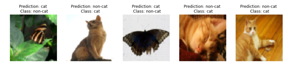
A few types of images the model tends to do poorly on include:

• Cat body in an unusual position
• Cat appears against a background of a similar color
• Unusual cat color and species
• Camera Angle
• Brightness of the picture
• Scale variation (cat is very large or small in image)

Congratulations on finishing this assignment!

You just built and trained a deep L-layer neural network, and applied it in order to distinguish cats from non-cats, a very serious and important task in deep learning. 😉

By now, you’ve also completed all the assignments for Course 1 in the Deep Learning Specialization. Amazing work! If you’d like to test out how closely you resemble a cat yourself, there’s an optional ungraded exercise below, where you can test your own image.

Great work and hope to see you in the next course!

7 - Test with your own image (optional/ungraded exercise)

From this point, if you so choose, you can use your own image to test the output of your model. To do that follow these steps:

1. Click on “File” in the upper bar of this notebook, then click “Open” to go on your Coursera Hub.
2. Add your image to this Jupyter Notebook’s directory, in the “images” folder
3. Change your image’s name in the following code
4. Run the code and check if the algorithm is right (1 = cat, 0 = non-cat)!

## START CODE HERE ##
my_image = "my_image.jpg" # change this to the name of your image file 
my_label_y = [1] # the true class of your image (1 -> cat, 0 -> non-cat)
## END CODE HERE ##

fname = "images/" + my_image
image = np.array(Image.open(fname).resize((num_px, num_px)))
plt.imshow(image)
image = image / 255.
image = image.reshape((1, num_px * num_px * 3)).T

my_predicted_image = predict(image, my_label_y, parameters)


print ("y = " + str(np.squeeze(my_predicted_image)) + ", your L-layer model predicts a \"" + classes[int(np.squeeze(my_predicted_image)),].decode("utf-8") +  "\" picture.")

Grades

后记

2024年5月11日20点完成Week 4，即完成这门课。从2024年5月9日到2024年5月11日花费3天的时间。因为是基础知识，所以学习理解起来比较快。这门课是吴恩达教授Deep Learning Specialization的第一门课，后续还有4门课程，希望有时间能够完成之。