简单演示一下基于卷积神经网络的信号解卷积,有个大致印象即可。
构造卷积滤波器
r = 0.9; % Define filter
om = 0.95;
a = [1 -2*r*cos(om) r^2];
b = [1 r*cos(om)];
h = filter(b, a, [zeros(1,38) 1 zeros(1,40)]);
N = 500;
K = 25;
sigma = 1;
绘制输入信号分量
set_plot_defaults('on')
hh = filter(b, a, [1 zeros(1,40)]);
groundtruth = zeros(1, N);
index_random = randperm(N);
index = index_random(1:K);
groundtruth(index) = 10*2*(rand(1,K) - 0.5);
after_conv = conv(groundtruth,h,'same');
noise = sigma * randn(1,N);
input = after_conv + noise;
figure(1)
subplot(2,2,1)
plot(1:N, groundtruth)
title('S[n]')
ylim([-10 10])
xlim([1,500])
box off
subplot(2,2,2)
plot(1:41, hh)
title('C[n]')
ylim([-1.2 1.8])
xlim([1,41])
box off
subplot(2,2,3)
plot(1:N, noise)
title('N[n]')
ylim([-10 10])
xlim([1,500])
box off
subplot(2,2,4)
plot(1:N, input)
title('x[n]')
ylim([-16 16])
xlim([1,500])
box off
加载3层解卷积CNN
load('sin2.mat');
deconvolver{1} = double(conv1);
deconvolver{2} = double(conv2);
deconvolver{3} = double(conv3);
% deconvolver{4} = double(conv4);
% deconvolver{5} = double(conv5);
绘制3层CNN的结构
set_plot_defaults('on')
figure(2)
[r,c,~] = size(deconvolver{1});
for i=1:1:r
for j=1:1:c
subplot(r,c,c*i-(c-j))
stem(flip(squeeze(deconvolver{1}(i,j,:))), 'filled', 'MarkerSize', 2)
hold on
plot(flip(squeeze(deconvolver{1}(i,j,:))))
hold off
xlim([0,18])
ylim([-1,1])
box off
end
end
sgtitle('layer1 (2x1)', 'FontSize', 10);
figure(3)
title('Layer 2')
[r,c,~] = size(deconvolver{2});
for i=1:1:r
for j=1:1:c
subplot(r,c,c*i-(c-j))
stem(flip(squeeze(deconvolver{2}(i,j,:))), 'filled', 'MarkerSize', 2)
hold on
plot(flip(squeeze(deconvolver{2}(i,j,:))))
hold off
xlim([0,38])
ylim([-0.25,inf])
box off
end
end
sgtitle('layer2 (2x2)', 'FontSize', 10);
figure(4)
title('Layer 3')
[r,c,~] = size(deconvolver{3});
for i=1:1:r
for j=1:1:c
subplot(r,c,c*i-(c-j))
stem(flip(squeeze(deconvolver{3}(i,j,:))), 'filled', 'MarkerSize', 2)
hold on
plot(flip(squeeze(deconvolver{3}(i,j,:))))
hold off
box off
end
end
sgtitle('layer3 (1x2)', 'FontSize', 10);
加载CNN
load('sin23_2.mat');
deconvolver{1} = double(conv1);
deconvolver{2} = double(conv2);
deconvolver{3} = double(conv3);
deconvolver{4} = double(conv4);
deconvolver{5} = double(conv5);
绘制CNN的第2层和第3层特征
set_plot_defaults('on')
figure(5)
[r,c,~] = size(deconvolver{2});
for i=1:1:r
for j=1:1:c
subplot(r,c,c*i-(c-j))
stem(flip(squeeze(deconvolver{2}(i,j,:))), 'filled', 'MarkerSize', 2)
hold on
plot(flip(squeeze(deconvolver{2}(i,j,:))))
hold off
xlim([1,17])
box off
end
end
sgtitle('layer2 (2x2)', 'FontSize', 10);
figure(6)
[r,c,~] = size(deconvolver{3});
for i=1:1:r
for j=1:1:c
subplot(r,c,c*i-(c-j))
stem(flip(squeeze(deconvolver{3}(i,j,:))), 'filled', 'MarkerSize', 2)
hold on
plot(flip(squeeze(deconvolver{3}(i,j,:))))
hold off
xlim([1,17])
box off
end
end
sgtitle('layer3 (2x2)', 'FontSize', 10);
绘制每一层的输出
groundtruth = zeros(1, N);
index_random = randperm(N);
index = index_random(1:K);
groundtruth(index) = 10*2*(rand(1,K) - 0.5);
after_conv = conv(groundtruth,h,'same');
noise = sigma * randn(1,N);
input = after_conv + noise;
figure(7)
plot(1:N, groundtruth)
title('The original sparse signal')
xlim([1,500])
ylim([-10,10])
box off
figure(8)
plot(1:N, input)
title('The input signal')
xlim([1,500])
ylim([-20,20])
box off
set_plot_defaults('on')
l1 = layer(input,deconvolver{1});
l2 = layer(l1,deconvolver{2});
l3 = layer(l2,deconvolver{3});
l4 = layer(l3,deconvolver{4});
output = CNN(input,deconvolver);
figure(9)
subplot(2,1,1)
plot(1:N, l1(1,:))
title('x_{1,1}[n]')
xlim([1,500])
ylim([-1,10])
box off
subplot(2,1,2)
plot(1:N, l1(2,:))
title('x_{1,2}[n]')
xlim([1,500])
ylim([-1,10])
box off
figure(10)
subplot(2,1,1)
plot(1:N, l3(1,:))
title('x_{3,1}[n]')
xlim([1,500])
ylim([-1,10])
box off
subplot(2,1,2)
plot(1:N, l3(2,:))
title('x_{3,2}[n]')
xlim([1,500])
ylim([-1,10])
box off
figure(11)
subplot(2,1,1)
plot(1:N, l4(1,:))
title('c_1[n]')
xlim([1,500])
ylim([-1,20])
box off
subplot(2,1,2)
plot(1:N, l4(2,:))
title('c_2[n]')
xlim([1,500])
ylim([-1,20])
box off
figure(12)
plot(1:N, output)
title('y[n]')
xlim([1,500])
ylim([-10,10])
box off
构造卷积滤波器并加载所提出的CNN
clc;
clear
r = 0.9; % Define filter
om = 0.95;
a = [1 -2*r*cos(om) r^2];
b = [1 r*cos(om)];
h = filter(b, a, [zeros(1,38) 1 zeros(1,40)]);
hh = filter(b, a, [1 zeros(1,40)]);
inverse = filter(1,hh,[zeros(1,36) 1 zeros(1,34)]);
load('sin23_2.mat');
deconvolver{1} = double(conv1);
deconvolver{2} = double(conv2);
deconvolver{3} = double(conv3);
deconvolver{4} = double(conv4);
deconvolver{5} = double(conv5);
构造测试信号
K = 25;
N = 500;
sigma = 0.5;
groundtruth = zeros(1, N);
index_random = randperm(N);
index = index_random(1:K);
groundtruth(index) = 10*2*(rand(1,K) - 0.5);
after_conv = conv(groundtruth,h,'same');
noise = sigma*randn(1,N);
input = after_conv + noise;
%% Plot input v.s. output in pure signal case
set_plot_defaults('on')
figure(13)
output = CNN(after_conv,deconvolver);
subplot(4,1,1)
plot(1:N, groundtruth)
xlim([1,500])
ylim([-10,10])
title('pure signal')
box off
subplot(4,1,2)
plot(1:N, after_conv)
xlim([1,500])
ylim([-15,15])
title('signal after convolution')
box off
subplot(4,1,3)
plot(1:N, after_conv)
xlim([1,500])
ylim([-15,15])
title('input signal')
box off
subplot(4,1,4)
plot(1:N, output)
xlim([1,500])
ylim([-10,10])
title('output signal')
box off
figure(14)
output1 = conv(after_conv,inverse,'same');
stem(1:N, groundtruth, 'b', 'MarkerSize', 4)
hold on
plot(1:N, output, 'ro', 'MarkerSize', 4)
hold on
plot(1:N, output1, 'gv', 'MarkerSize', 4)
hold off
legend('pure sparse signal', 'output of CNN','output of inverse filter')
box off
figure(15)
output = CNN(noise,deconvolver);
subplot(4,1,1)
plot(1:N, zeros(1,N))
xlim([1,500])
ylim([-2,2])
title('pure signal')
box off
subplot(4,1,2)
plot(1:N, zeros(1,N))
xlim([1,500])
ylim([-2,2])
title('signal after convolution')
box off
subplot(4,1,3)
plot(1:N, noise)
xlim([1,500])
ylim([-2,2])
title('input signal')
box off
subplot(4,1,4)
plot(1:N, output)
xlim([1,500])
ylim([-2,2])
title('output signal')
box off
%
figure(16)
output1 = conv(noise,inverse,'same');
stem(1:N, zeros(1,N), 'b', 'MarkerSize', 4)
hold on
plot(1:N, output, 'ro', 'MarkerSize', 4)
hold on
plot(1:N, output1, 'gv', 'MarkerSize', 4)
hold off
legend('pure sparse signal', 'output of CNN','output of inverse filter')
box off
figure(17)
output = CNN(input,deconvolver);
subplot(4,1,1)
plot(1:N, groundtruth)
xlim([1,500])
ylim([-10,10])
title('pure signal')
box off
subplot(4,1,2)
plot(1:N, after_conv)
xlim([1,500])
ylim([-15,15])
title('signal after convolution')
box off
subplot(4,1,3)
plot(1:N, input)
xlim([1,500])
ylim([-15,15])
title('input signal')
box off
subplot(4,1,4)
plot(1:N, output)
xlim([1,500])
ylim([-10,10])
title('output signal')
box off
figure(18)
output1 = conv(input,inverse,'same');
stem(1:N, groundtruth, 'b', 'MarkerSize', 4)
hold on
plot(1:N, output, 'ro', 'MarkerSize', 4)
hold on
plot(1:N, output1, 'gv', 'MarkerSize', 4)
hold off
legend('pure sparse signal', 'output of CNN','output of inverse filter')
box off
%% Create input signal (noisy signal) and ground truth (pure signal) for the performance part.
% N is the total length of the pure sparse signal.
% K is the number of non-zeros in the pure sparse signal.
% As a result, 1-K/N determines the sparsity of the pure signal.
N = 500;
num = 2000;
sigma_set = logspace(log10(0.1), log10(2), 20);
% sigma_set = 0.1:0.1:2;
MSE_output_ave = zeros(3,length(sigma_set));
SNR_output_ave = zeros(3,length(sigma_set));
for m = 1:1:3
K = 25 * m;
for i = 1:1:length(sigma_set)
sigma = sigma_set(i);
SNR_output = zeros(1,num);
SNR_input = zeros(1,num);
MSE_output = zeros(1,num);
for j = 1:1:num
groundtruth = zeros(1, N);
index_random = randperm(N);
index = index_random(1:K);
groundtruth(index) = 10*2*(rand(1,K) - 0.5);
% groundtruth(index) = 10*randn(1,K);
after_conv = conv(groundtruth,h,'same');
input_noise = sigma*randn(1,N);
input = after_conv + input_noise;
output = CNN(input, deconvolver);
noise = output - groundtruth;
MSE_output(j) = mean(noise.^2);
SNR_output(j) = 10*log10(mean(groundtruth.^2)/MSE_output(j));
end
SNR_output_ave(m,i) = mean(SNR_output);
% MSE_output_ave(m,i) = mean(MSE_output);
MSE_output_ave(m,i) = sqrt(mean(MSE_output));
end
end
%% Plot the performance v.s. sparsity and noise level
set_plot_defaults('on')
figure(19)
semilogx(sigma_set,SNR_output_ave(1,:),'r.-',sigma_set,SNR_output_ave(2,:),'k.-',sigma_set,SNR_output_ave(3,:),'g.-')
legend('Sparsity = 95%','Sparsity = 90%','Sparsity = 85%')
xlabel('σ')
ylabel('SNR in dB')
set(gca, 'xtick', [0.1 0.2 0.5 1 2.0])
xlim([min(sigma_set) max(sigma_set)])
box off
figure(20)
semilogx(sigma_set,MSE_output_ave(1,:),'r.-',sigma_set,MSE_output_ave(2,:),'k.-',sigma_set,MSE_output_ave(3,:),'g.-')
legend('Output RMSE, sparsity = 95%','Output RMSE, sparsity = 90%','Output RMSE, sparsity = 85%', 'Location','NorthWest')
xlabel('σ')
ylabel('RMSE')
set(gca, 'xtick', [0.1 0.2 0.5 1 2.0])
xlim([min(sigma_set) max(sigma_set)])
box off
工学博士,担任《Mechanical System and Signal Processing》《中国电机工程学报》等期刊审稿专家,擅长领域:现代信号处理,机器学习/深度学习,时间序列分析/预测,设备智能故障诊断与健康管理PHM等。