Using LoRA for efficient fine-tuning: Fundamental principles — ROCm Blogs (amd.com)
大型语言模型的低秩适配(LoRA)用于解决微调大型语言模型(LLMs)的挑战。GPT和Llama等拥有数十亿参数的模型,特定任务或领域的微调通常成本高昂。LoRA保留了预训练模型权重,并在每个模型块内添加可训练层。这显著减少了需要微调的参数数量,并大幅减少了GPU内存需求。LoRA的关键优势在于它大大减少了可训练参数的数量——有时高达10000倍——从而显著减少了GPU资源的需求。
为何LoRA有效
预训练的LLMs在适应新任务时具有较低的“内在维度”,这意味着数据可以通过较低维度的空间有效表示或近似,同时保留其大部分关键信息或结构。我们可以将适应特定任务后的新权重矩阵分解成低维(更小的)矩阵,而不会丢失太多重要信息。这是通过低秩近似来实现的。
矩阵的秩是一个值,它给出了矩阵复杂性的一个概念。低秩近似旨在尽可能接近地近似原始矩阵,但具有较低的秩。低秩矩阵降低了计算复杂性,因此提高了矩阵乘法的效率。低秩分解指的是通过导出矩阵A的低秩近似来有效地近似矩阵A的过程。奇异值分解(SVD)是一种常用的低秩分解方法。
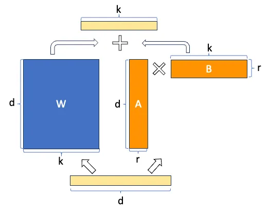
假设`W`代表给定神经网络层中的权重矩阵,假设`ΔW`是`W`在完全微调后的权重更新。然后我们可以将权重更新矩阵`ΔW`分解为两个较小的矩阵:`ΔW = WA*WB`,其中`WA`是一个`A × r`维的矩阵,`WB`是一个`r × B`维的矩阵。这里,我们保持原始权重`W`固定,只训练新的矩阵`WA`和`WB`。这概括了LoRA方法,如下图所示。
LoRA 的好处
• 降低资源消耗。 微调深度学习模型通常需要大量的计算资源,这可能既昂贵又耗时。LoRA在保持高性能的同时减少了资源的需求。
• 加快迭代速度。 LoRA 使得快速迭代成为可能,便于尝试不同的微调任务并快速适配模型。
• 改进迁移学习。 LoRA 提升了迁移学习的效能,因为应用了LoRA适配器的模型可以通过更少的数据完成微调。这在标记数据稀缺的情况下特别有价值。
• 广泛的适用性。 LoRA 具有多样性,可以被应用于包括自然语言处理、计算机视觉与语音识别等多个领域。
• 降低碳足迹。 通过减少计算需求,LoRA 为深度学习贡献了一种更绿色、更可持续的方法。
使用LoRA技术训练神经网络
在这篇博客中,我们使用 CIFAR-10 数据集训练了一个基础的图像分类器,从零开始经过几个时期的训练。之后,我们应用了LoRA继续对模型进行训练,演示了在训练过程中加入LoRA的优势。
设置
此演示使用以下设置创建。有关详细的支持信息,请参见 ROCm 文档。
- 硬件和操作系统:
- AMD Instinct GPU
- Ubuntu 22.04.3 LTS
- 软件:
- ROCm 5.7.0+
- Pytorch 2.0+
入门
1. 导入包。
import torch
import torchvision
import torchvision.transforms as transforms
2. 加载数据集并设置设备。
# 来自CIFAR10数据集的10个类别
classes = ('airplane', 'automobile', 'bird', 'cat', 'deer', 'dog', 'frog', 'horse', 'ship', 'truck')

# 批量大小
batch_size = 8

# 图像预处理
preprocessor = transforms.Compose(
    [transforms.ToTensor(),
    transforms.Normalize((0.5, 0.5, 0.5), (0.5, 0.5, 0.5))])

# 训练数据集
train_set = torchvision.datasets.CIFAR10(root='./dataset', train=True,
                                        download=True, transform=preprocessor)
train_loader = torch.utils.data.DataLoader(train_set, batch_size=batch_size,
                                        shuffle=True, num_workers=8)
#  测试数据集
test_set = torchvision.datasets.CIFAR10(root='./dataset', train=False,
                                    download=True, transform=preprocessor)
test_loader = torch.utils.data.DataLoader(test_set, batch_size=batch_size,
                                        shuffle=False, num_workers=8)

# 定义设备
device = torch.device("cuda:0" if torch.cuda.is_available() else "cpu")
3. 展示数据集中的一些样本。
import matplotlib.pyplot as plt
import numpy as np
# 辅助函数显示图像
def image_display(images):
# 获取原始图像
images = images * 0.5 + 0.5
plt.imshow(np.transpose(images.numpy(), (1, 2, 0)))
plt.axis('off')
plt.show()
# 获取一批图像
images, labels = next(iter(train_loader))
# 展示图像
image_display(torchvision.utils.make_grid(images))
# 显示实际标签
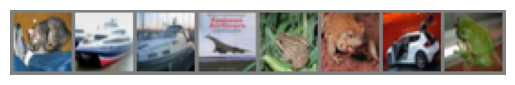
print('Ground truth labels: ', ' '.join(f'{classes[labels[j]]}' for j in range(images.shape[0])))输出:

真实标签:猫 船 船 飞机 青蛙 青蛙 汽车 青蛙(在机器学习和深度学习领域,"Ground truth" 是一个常见的术语,指的是在训练或测试模型时使用的真实标签或目标值。它是一个标准或参考,用来衡量模型预测的准确性。具体来说:
- Ground:在这个上下文中,"ground" 并不是指地面,而是指基础或根本的意思。
- Truth:指的是真实的标签或目标值。
因此,"Ground truth labels" 可以理解为“基础的真实标签”或“参考的真实标签”。在翻译成中文时,通常简化为“真实标签”,以便更容易理解。
总的来说,"Ground truth" 在这个领域的意思是用来作为模型评估标准的真实数据。)
4. 创建一个基本的三层神经网络用于图像分类,侧重于简单性,以清晰地阐释LoRA的效果。
import torch.nn as nn
import torch.nn.functional as F

class net(nn.Module):
    def __init__(self):
        super().__init__()
        self.fc1 = nn.Linear(3*32*32, 4096)
        self.fc2 = nn.Linear(4096, 2048)
        self.fc3 = nn.Linear(2048, 10)

    def forward(self, x):
        x = torch.flatten(x, 1)
        x = F.relu(self.fc1(x))
        x = F.relu(self.fc2(x))
        x = self.fc3(x)
        return x

# 将模型移动到设备上
classifier = net().to(device)
5. 训练模型。
import torch.optim as optim

def train(train_loader, classifier, start_epoch = 0, epochs=1, device="cuda:0"):
    classifier = classifier.to(device)
    classifier.train()
    criterion = nn.CrossEntropyLoss()
    optimizer = optim.Adam(classifier.parameters(), lr=0.001)

    for epoch in range(epochs):  # 训练循环

        loss_log = 0.0
        for i, data in enumerate(train_loader, 0):
            inputs, labels = data[0].to(device), data[1].to(device)
            # 重置参数梯度
            optimizer.zero_grad()

            outputs = classifier(inputs)
            loss = criterion(outputs, labels)
            loss.backward()
            optimizer.step()

            # 在每1000个小批次之后打印损失
            loss_log += loss.item()
            if i % 2000 == 1999:
                print(f'[{start_epoch + epoch}, {i+1:5d}] loss: {loss_log / 2000:.3f}')
                loss_log = 0.0
开始训练模型。
import time

start_epoch = 0
epochs = 1
# 用一个epoch预热GPU
train(train_loader, classifier, start_epoch=start_epoch, epochs=epochs, device=device)

# 运行另一个epoch记录时间
start_epoch += epochs
epochs = 1
start = time.time()
train(train_loader, classifier, start_epoch=start_epoch, epochs=epochs, device=device)
torch.cuda.synchronize()
end = time.time()
train_time = (end - start)

print(f"One epoch takes {train_time:.3f} seconds")
输出:
    [0,  2000] loss: 1.987
    [0,  4000] loss: 1.906
    [0,  6000] loss: 1.843
    [1,  2000] loss: 1.807
    [1,  4000] loss: 1.802
    [1,  6000] loss: 1.782
    One epoch takes 31.896 seconds
一个epoch大约需要31秒。
保存模型。
model_path = './classifier_cira10.pth'
torch.save(classifier.state_dict(), model_path)
我们稍后会训练同样的模型,并应用LoRA,检查使用一个epoch训练需要多长时间。
6. 加载已保存的模型并进行快速测试。
# 准备测试数据。
images, labels = next(iter(test_loader))
# 展示测试图片
image_display(torchvision.utils.make_grid(images))
# 显示真实标签
print('Ground truth labels: ', ' '.join(f'{classes[labels[j]]}' for j in range(images.shape[0])))

# 加载已保存的模型并进行测试
model = net()
model.load_state_dict(torch.load(model_path))
model = model.to(device)
images = images.to(device)
outputs = model(images)
_, predicted = torch.max(outputs, 1)

print('Predicted: ', ' '.join(f'{classes[predicted[j]]}'
                            for j in range(images.shape[0])))
输出:

真实标签: 猫 船 船 飞机 青蛙 青蛙 汽车 青蛙
预测: 鹿 卡车 飞机 船 鹿 青蛙 汽车 鸟
我们观察到,仅训练模型两个周期并没有产生满意的结果。让我们检查一下模型在整个测试数据集上的表现。
def test(model, test_loader, device):
    model=model.to(device)
    model.eval()
    correct = 0
    total = 0
    with torch.no_grad():
        for data in test_loader:
            images, labels = data[0].to(device), data[1].to(device)
            # images = images.to(device)
            # labels = labels.to(device)
            # inference
            outputs = model(images)
            # 获取最佳预测结果
            _, predicted = torch.max(outputs.data, 1)

            total += labels.size(0)
            correct += (predicted == labels).sum().item()

    print(f'Accuracy of the given model on the {total} test images is {100 * correct // total} %')

test(model, test_loader, device)
输出:
Accuracy of the given model on the 10000 test images is 32 %这个结果表明,通过进一步训练,模型有很大的改进潜力。在接下来的章节中,我们将应用LoRA到模型,并继续使用这种方法进行训练。
7. 将LoRA应用到模型上。
定义一些辅助函数来将LoRA应用到模型上。
class ParametrizationWithLoRA(nn.Module):
    def __init__(self, features_in, features_out, rank=1, alpha=1, device='cpu'):
        super().__init__()

        # Create A B and scale used in ∆W = BA x α/r
        self.lora_weights_A = nn.Parameter(torch.zeros((rank,features_out)).to(device))
        nn.init.normal_(self.lora_weights_A, mean=0, std=1)
        self.lora_weights_B = nn.Parameter(torch.zeros((features_in, rank)).to(device))
        self.scale = alpha / rank

        self.enabled = True

    def forward(self, original_weights):
        if self.enabled:
            return original_weights + torch.matmul(self.lora_weights_B, self.lora_weights_A).view(original_weights.shape) * self.scale
        else:
            return original_weights

def apply_parameterization_lora(layer, device, rank=1, alpha=1):
    """
    Apply loRA to a given layer
    """
    features_in, features_out = layer.weight.shape
    return ParametrizationWithLoRA(
        features_in, features_out, rank=rank, alpha=alpha, device=device
    )

def enable_lora(model, enabled=True):
    """
    enabled = True: incorporate the the lora parameters to the model
    enabled = False: the lora parameters have no impact on the model
    """
    for layer in [model.fc1, model.fc2, model.fc3]:
        layer.parametrizations["weight"][0].enabled = enabled
将LoRA应用到我们的模型中。
import torch.nn.utils.parametrize as parametrize
parametrize.register_parametrization(model.fc1, "weight", apply_parameterization_lora(model.fc1, device))
parametrize.register_parametrization(model.fc2, "weight", apply_parameterization_lora(model.fc2, device))
parametrize.register_parametrization(model.fc3, "weight", apply_parameterization_lora(model.fc3, device))
现在,我们的模型的参数包括两部分:原始参数和通过LoRA引入的参数。由于我们尚未训练这个更新后的模型,LoRA的权重被初始化了,不应该影响模型的精确度(参考‘ParametrizationWithLoRA')。因此,禁用或启用LoRA,模型的精确度应该是相同的。让我们来测试这个假设。
enable_lora(model, enabled=False)
test(model, test_loader, device)
输出结果:
Accuracy of the network on the 10000 test images: 32 %enable_lora(model, enabled=True)
test(model, test_loader, device)输出结果:
Accuracy of the network on the 10000 test images: 32 %这是我们预期的结果。
现在让我们看看LoRA增加了多少参数。
total_lora_params = 0
total_original_params = 0
for index, layer in enumerate([model.fc1, model.fc2, model.fc3]):
total_lora_params += layer.parametrizations["weight"][0].lora_weights_A.nelement() + layer.parametrizations["weight"][0].lora_weights_B.nelement()
total_original_params += layer.weight.nelement() + layer.bias.nelement()
print(f'Number of parameters in the model with LoRA: {total_lora_params + total_original_params:,}')
print(f'Parameters added by LoRA: {total_lora_params:,}')
params_increment = (total_lora_params / total_original_params) * 100
print(f'Parameters increment: {params_increment:.3f}%')输出结果:
带LoRA的模型中的参数数量: 21,013,524
LoRA添加的参数: 15,370
参数增长: 0.073%LoRA仅为我们的模型增加了0.073%的参数。
8. 继续用LoRA训练模型
在我们继续训练模型之前,我们想要根据文章所说冻结所有模型的原始参数。通过这样做,我们只更新由LoRA引入的权重,这是原始模型参数数量的0.073%。
for name, param in model.named_parameters():
if 'lora' not in name:
param.requires_grad = False使用LoRA继续训练模型。
# 确保启用了LoRA
enable_lora(model, enabled=True)
start_epoch += epochs
epochs = 1
# warm up the GPU with the new model (loRA enabled) one epoch for testing the training time
train(train_loader, model, start_epoch=start_epoch, epochs=epochs, device=device)
start = time.time()
# 运行另一个周期以记录时间
start_epoch += epochs
epochs = 1
import time
start = time.time()
train(train_loader, model, start_epoch=start_epoch, epochs=epochs, device=device)
torch.cuda.synchronize()
end = time.time()
train_time = (end - start)
print(f"One epoch takes {train_time} seconds")输出结果:
[2, 2000] loss: 1.643
[2, 4000] loss: 1.606
[2, 6000] loss: 1.601
[3, 2000] loss: 1.568
[3, 4000] loss: 1.560
[3, 6000] loss: 1.585
One epoch takes 16.622623205184937 seconds你可能注意到,现在完成一个训练周期大约只需要16秒钟,这大约是训练原始模型所需时间的53%(31秒)。
损失的减少意味着模型已经通过更新LoRA引入的参数学到了一些东西。现在,如果我们启用LoRA来测试模型,准确度应该高于我们之前使用原始模型获得的32%。如果我们禁用LoRA,模型应该会产生和原始模型相同的准确率。让我们继续进行这些测试。
enable_lora(model, enabled=True)
test(model, test_loader, device)
enable_lora(model, enabled=False)
test(model, test_loader, device)输出结果:
    给定模型在10000张测试图片上的准确率为 42 %
    给定模型在10000张测试图片上的准确率为 32 %
用之前的图片再次测试更新后的模型。
# 展示测试图片
image_display(torchvision.utils.make_grid(images.cpu()))
# 展示真实标签
print('Ground truth labels: ', ' '.join(f'{classes[labels[j]]}' for j in range(images.shape[0])))

# 载入保存好的模型并进行测试
enable_lora(model, enabled=True)
images = images.to(device)
outputs = model(images)
_, predicted = torch.max(outputs, 1)

print('Predicted: ', ' '.join(f'{classes[predicted[j]]}'
                            for j in range(images.shape[0])))
输出:
真实标签:猫 船 船 飞机 青蛙 青蛙 汽车 青蛙
预测:猫 船 船 船 青蛙 青蛙 汽车 青蛙
我们可以观察到,与第六步得到的结果相比,新模型的表现更好,证明了参数确实学习到了有意义的信息。
结论
在这篇博客文章中,我们探讨了LoRA算法,深入研究了其原理和在AMD GPU上使用ROCm实现的方法。我们从头开始开发了一个基本的网络和LoRA模块,以展示LoRA如何有效地减少可训练参数和训练时间。我们邀请您通过阅读有关使用LoRA微调Llama 2模型和在单个AMD GPU上使用QLoRA微调Llama 2的更多内容来深入了解。