tensorflow之欠拟合与过拟合，正则化缓解

过拟合泛化性弱

欠拟合解决方法：

        增加输入特征项

        增加网络参数

        减少正则化参数

过拟合的解决方法：

        数据清洗

        增大训练集

        采用正则化

        增大正则化参数

正则化缓解过拟合

正则化在损失函数中引入模型复杂度指标，利用给w增加权重，弱化数据集的噪声，loss = loss(y与y_) + REGULARIZER*loss(w)

模型中所有参数的损失函数，如交叉上海，均方误差

利用超参数REGULARIZER给出参数w在总loss中的比例，即正则化权重， w是需要正则化的参数

正则化的选择

L1正则化大概率会使很多参数变为0，因此该方法可通过系数参数，减少参数的数量，降低复杂度

L2正则化会使参数很接近0但不为0，因此该方法可通过减少参数值的大小降低复杂度 

with tf.GradientTape() as tape:
    h1 = tf.matul(x_train, w1) + b1
    h1 = tf.nn.relu(h1)
    y = tf.matmul(h1, w2) + b2
    loss_mse = tf.reduce_mean(tf.square(y_train - y))
    loss_ragularization = []
    loss_regularization.append(tf.nn.l2_loss(w1))
    loss_regularization.append(tf.nn.l2_loss(w2))
    loss_regularization = tf.reduce_sum(loss_regularization)
    loss = loss_mse + 0.03 * loss_regularization
variables = [w1, b1, w2, b2】
grads = tape.gradient(loss, variables)

生成网格覆盖这些点，会对每个坐标生成一个预测值，输出预测值为0.5的连成线，这个线就是红点和蓝点的分界线。

# 导入所需模块
import tensorflow as tf
from matplotlib import pyplot as plt
import numpy as np
import pandas as pd

# 读入数据/标签 生成x_train y_train
df = pd.read_csv('dot.csv')
x_data = np.array(df[['x1', 'x2']])
y_data = np.array(df['y_c'])

x_train = x_data
y_train = y_data.reshape(-1, 1)

Y_c = [['red' if y else 'blue'] for y in y_train]

# 转换x的数据类型，否则后面矩阵相乘时会因数据类型问题报错
x_train = tf.cast(x_train, tf.float32)
y_train = tf.cast(y_train, tf.float32)

# from_tensor_slices函数切分传入的张量的第一个维度，生成相应的数据集，使输入特征和标签值一一对应
train_db = tf.data.Dataset.from_tensor_slices((x_train, y_train)).batch(32)

# 生成神经网络的参数，输入层为4个神经元，隐藏层为32个神经元，2层隐藏层，输出层为3个神经元
# 用tf.Variable()保证参数可训练
w1 = tf.Variable(tf.random.normal([2, 11]), dtype=tf.float32)
b1 = tf.Variable(tf.constant(0.01, shape=[11]))

w2 = tf.Variable(tf.random.normal([11, 1]), dtype=tf.float32)
b2 = tf.Variable(tf.constant(0.01, shape=[1]))

lr = 0.005  # 学习率为
epoch = 800  # 循环轮数

# 训练部分
for epoch in range(epoch):
    for step, (x_train, y_train) in enumerate(train_db):
        with tf.GradientTape() as tape:  # 记录梯度信息

            h1 = tf.matmul(x_train, w1) + b1  # 记录神经网络乘加运算
            h1 = tf.nn.relu(h1)
            y = tf.matmul(h1, w2) + b2

            # 采用均方误差损失函数mse = mean(sum(y-out)^2)
            loss_mse = tf.reduce_mean(tf.square(y_train - y))
            # 添加l2正则化
            loss_regularization = []
            # tf.nn.l2_loss(w)=sum(w ** 2) / 2
            loss_regularization.append(tf.nn.l2_loss(w1))
            loss_regularization.append(tf.nn.l2_loss(w2))
            # 求和
            # 例：x=tf.constant(([1,1,1],[1,1,1]))
            #   tf.reduce_sum(x)
            # >>>6
            loss_regularization = tf.reduce_sum(loss_regularization)
            loss = loss_mse + 0.03 * loss_regularization  # REGULARIZER = 0.03

        # 计算loss对各个参数的梯度
        variables = [w1, b1, w2, b2]
        grads = tape.gradient(loss, variables)

        # 实现梯度更新
        # w1 = w1 - lr * w1_grad
        w1.assign_sub(lr * grads[0])
        b1.assign_sub(lr * grads[1])
        w2.assign_sub(lr * grads[2])
        b2.assign_sub(lr * grads[3])

    # 每200个epoch，打印loss信息
    if epoch % 20 == 0:
        print('epoch:', epoch, 'loss:', float(loss))

# 预测部分
print("*******predict*******")
# xx在-3到3之间以步长为0.01，yy在-3到3之间以步长0.01,生成间隔数值点
xx, yy = np.mgrid[-3:3:.1, -3:3:.1]
# 将xx, yy拉直，并合并配对为二维张量，生成二维坐标点
grid = np.c_[xx.ravel(), yy.ravel()]
grid = tf.cast(grid, tf.float32)
# 将网格坐标点喂入神经网络，进行预测，probs为输出
probs = []
for x_predict in grid:
    # 使用训练好的参数进行预测
    h1 = tf.matmul([x_predict], w1) + b1
    h1 = tf.nn.relu(h1)
    y = tf.matmul(h1, w2) + b2  # y为预测结果
    probs.append(y)

# 取第0列给x1，取第1列给x2
x1 = x_data[:, 0]
x2 = x_data[:, 1]
# probs的shape调整成xx的样子
probs = np.array(probs).reshape(xx.shape)
plt.scatter(x1, x2, color=np.squeeze(Y_c))
# 把坐标xx yy和对应的值probs放入contour函数，给probs值为0.5的所有点上色  plt.show()后 显示的是红蓝点的分界线
plt.contour(xx, yy, probs, levels=[.5])
plt.show()

# 读入红蓝点，画出分割线，包含正则化
# 不清楚的数据，建议print出来查看

存在过拟合现象，轮廓不够平滑， 使用l2正则化缓解过拟合

# 导入所需模块
import tensorflow as tf
from matplotlib import pyplot as plt
import numpy as np
import pandas as pd

# 读入数据/标签 生成x_train y_train
df = pd.read_csv('dot.csv')
x_data = np.array(df[['x1', 'x2']])
y_data = np.array(df['y_c'])

x_train = x_data
y_train = y_data.reshape(-1, 1)

Y_c = [['red' if y else 'blue'] for y in y_train]

# 转换x的数据类型，否则后面矩阵相乘时会因数据类型问题报错
x_train = tf.cast(x_train, tf.float32)
y_train = tf.cast(y_train, tf.float32)

# from_tensor_slices函数切分传入的张量的第一个维度，生成相应的数据集，使输入特征和标签值一一对应
train_db = tf.data.Dataset.from_tensor_slices((x_train, y_train)).batch(32)

# 生成神经网络的参数，输入层为4个神经元，隐藏层为32个神经元，2层隐藏层，输出层为3个神经元
# 用tf.Variable()保证参数可训练
w1 = tf.Variable(tf.random.normal([2, 11]), dtype=tf.float32)
b1 = tf.Variable(tf.constant(0.01, shape=[11]))

w2 = tf.Variable(tf.random.normal([11, 1]), dtype=tf.float32)
b2 = tf.Variable(tf.constant(0.01, shape=[1]))

lr = 0.005  # 学习率为
epoch = 800  # 循环轮数

# 训练部分
for epoch in range(epoch):
    for step, (x_train, y_train) in enumerate(train_db):
        with tf.GradientTape() as tape:  # 记录梯度信息

            h1 = tf.matmul(x_train, w1) + b1  # 记录神经网络乘加运算
            h1 = tf.nn.relu(h1)
            y = tf.matmul(h1, w2) + b2

            # 采用均方误差损失函数mse = mean(sum(y-out)^2)
            loss_mse = tf.reduce_mean(tf.square(y_train - y))
            # 添加l2正则化
            loss_regularization = []
            # tf.nn.l2_loss(w)=sum(w ** 2) / 2
            loss_regularization.append(tf.nn.l2_loss(w1))
            loss_regularization.append(tf.nn.l2_loss(w2))
            # 求和
            # 例：x=tf.constant(([1,1,1],[1,1,1]))
            #   tf.reduce_sum(x)
            # >>>6
            loss_regularization = tf.reduce_sum(loss_regularization)
            loss = loss_mse + 0.03 * loss_regularization  # REGULARIZER = 0.03

        # 计算loss对各个参数的梯度
        variables = [w1, b1, w2, b2]
        grads = tape.gradient(loss, variables)

        # 实现梯度更新
        # w1 = w1 - lr * w1_grad
        w1.assign_sub(lr * grads[0])
        b1.assign_sub(lr * grads[1])
        w2.assign_sub(lr * grads[2])
        b2.assign_sub(lr * grads[3])

    # 每200个epoch，打印loss信息
    if epoch % 20 == 0:
        print('epoch:', epoch, 'loss:', float(loss))

# 预测部分
print("*******predict*******")
# xx在-3到3之间以步长为0.01，yy在-3到3之间以步长0.01,生成间隔数值点
xx, yy = np.mgrid[-3:3:.1, -3:3:.1]
# 将xx, yy拉直，并合并配对为二维张量，生成二维坐标点
grid = np.c_[xx.ravel(), yy.ravel()]
grid = tf.cast(grid, tf.float32)
# 将网格坐标点喂入神经网络，进行预测，probs为输出
probs = []
for x_predict in grid:
    # 使用训练好的参数进行预测
    h1 = tf.matmul([x_predict], w1) + b1
    h1 = tf.nn.relu(h1)
    y = tf.matmul(h1, w2) + b2  # y为预测结果
    probs.append(y)

# 取第0列给x1，取第1列给x2
x1 = x_data[:, 0]
x2 = x_data[:, 1]
# probs的shape调整成xx的样子
probs = np.array(probs).reshape(xx.shape)
plt.scatter(x1, x2, color=np.squeeze(Y_c))
# 把坐标xx yy和对应的值probs放入contour函数，给probs值为0.5的所有点上色  plt.show()后 显示的是红蓝点的分界线
plt.contour(xx, yy, probs, levels=[.5])
plt.show()

# 读入红蓝点，画出分割线，包含正则化
# 不清楚的数据，建议print出来查看

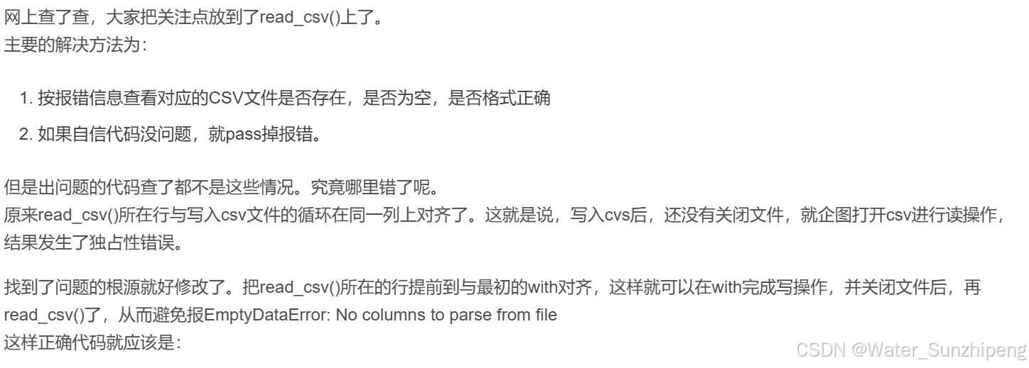
python EmptyDataError No columns to parse from file sites:stackoverflow.com