首先导入数据
import numpy as np
from scipy.integrate import odeint
from scipy.optimize import minimize
import matplotlib.pyplot as plt

data = np.array([
    [30, 4],
    [47.2, 6.1],
    [70.2, 9.8],
    [77.4, 35.2],
    [36.3, 59.4],
    [20.6, 41.7],
    [18.1, 19],
    [21.4, 13],
    [22, 8.3],
    [25.4, 9.1],
    [27.1, 7.4],
    [40.3, 8],
    [57, 12.3],
    [76.6, 19.5],
    [52.3, 45.7],
    [19.5, 51.1],
    [11.2, 29.7],
    [7.6, 15.8],
    [14.6, 9.7],
    [16.2, 10.1],
    [24.7, 8.6]
])
设置参数和定义函数
# Set initial parameters to small random values or default values
initial_guess = [0.1, 0.1, 0.1, 0.1, 0.1, 0.1]

# Define ordinary differential equations
def model(y, t, a, b, c, d, e, f):
    x, z = y
    dxdt = a * x - b * x * z - e * x**2
    dydt = -c * z + d * x * z - f * z**2
    return [dxdt, dydt]

#Define error function
def error(params):
    a, b, c, d, e, f = params
    t = np.linspace(0, 1, len(data))
    y0 = [data[0, 0], data[0, 1]]
    y_pred = odeint(model, y0, t, args=(a, b, c, d, e, f))
    x_pred, z_pred = y_pred[:, 0], y_pred[:, 1]
    error_x = np.sum((x_pred - data[:, 0])**2)
    error_y = np.sum((z_pred - data[:, 1])**2)
    total_error = error_x + error_y
    return total_error

# Use least squares method to fit parameters
result = minimize(error, initial_guess, method='Nelder-Mead')

# Get the fitting parameter values
a_fit, b_fit, c_fit, d_fit, e_fit, f_fit = result.x

# Simulate the fitted trajectory
t_fit = np.linspace(0, 1, len(data))
y0_fit = [data[0, 0], data[0, 1]]
y_fit = odeint(model, y0_fit, t_fit, args=(a_fit, b_fit, c_fit, d_fit, e_fit, f_fit))
x_fit, z_fit = y_fit[:, 0], y_fit[:, 1]

# Plot the fitting results against the original data points
plt.figure(figsize=(10, 6))
plt.scatter(data[:, 0], data[:, 1], label='Raw data', marker='o', color='blue')
plt.plot(x_fit, z_fit, label='Fitting results', linestyle='-', color='red')
plt.xlabel('x')
plt.ylabel('y')
plt.legend()
plt.grid()
plt.show() 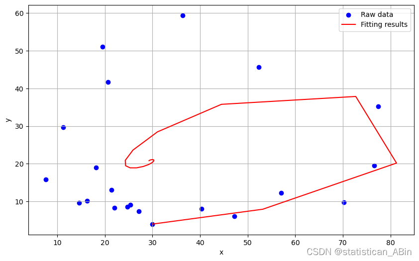
进一步优化
import matplotlib.pyplot as plt


# Different optimization methods
methods = ['Nelder-Mead', 'Powell', 'BFGS', 'L-BFGS-B']

for method in methods:
    result = minimize(error, initial_guess, method=method)
    a_fit, b_fit, c_fit, d_fit, e_fit, f_fit = result.x

  # Simulate the fitted trajectory
    t_fit = np.linspace(0, 1, len(data))
    y0_fit = [data[0, 0], data[0, 1]]
    y_fit = odeint(model, y0_fit, t_fit, args=(a_fit, b_fit, c_fit, d_fit, e_fit, f_fit))
    x_fit, z_fit = y_fit[:, 0], y_fit[:, 1]

# Plot the fitting results against the original data points
    plt.figure(figsize=(10, 6))
    plt.scatter(data[:, 0], data[:, 1], label='Raw data', marker='o', color='blue')
    plt.plot(x_fit, z_fit, label=f'Fitting results ({method})', linestyle='-', color='red')
    plt.xlabel('x')
    plt.ylabel('y')
    plt.legend()
    plt.grid()
    plt.show()

print(f"Parameter values fitted using {method} method:a={a_fit}, b={b_fit}, c={c_fit}, d={d_fit}, e={e_fit}, f={f_fit}") 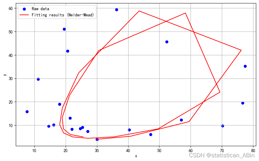
Parameter values fitted using Nelder-Mead method:a=1.2173283165346425, b=0.42516102725023064, c=19.726779624261006, d=0.7743814851338301, e=-0.19482192444374966, f=0.37455729849779884
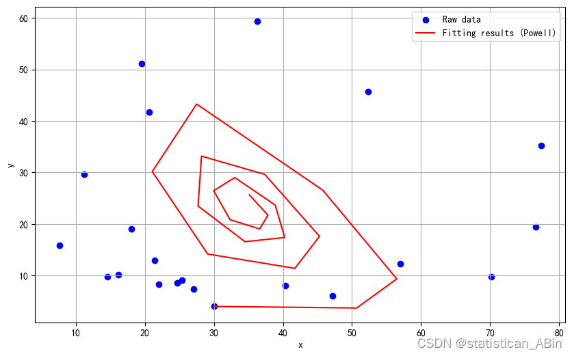
Parameter values fitted using Powell method:a=32.49329459442917, b=0.6910719576651617, c=58.98701472032894, d=1.3524516626786816, e=0.47787798383104335, f=-0.5344483269192019
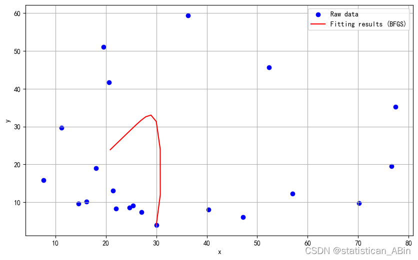
Parameter values fitted using BFGS method:a=1.2171938888848015, b=0.04968374479958104, c=0.9234835772585344, d=0.947268540340848, e=0.010742224447412019, f=0.7985132960108715
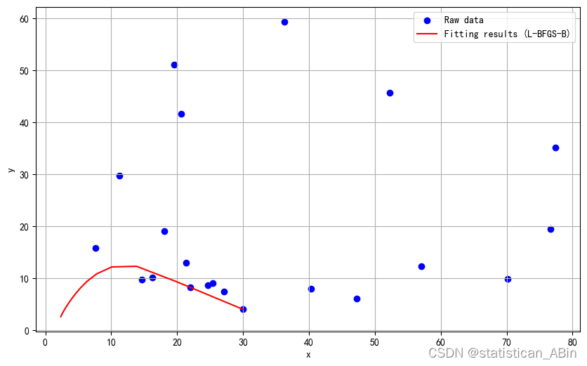
Parameter values fitted using L-BFGS-B method:a=1.154759061832585, b=0.32168624538800344, c=0.9455699334793284, d=0.9623931795647013, e=0.2936335531513881, f=0.8566315817923148
进一步优化
#Set parameter search range (interval)
bounds = [(-5, 25), (-5, 25), (-5, 25), (-5, 25), (-5, 25), (-5, 25)]

# Use interval search to set initial parameter values
result = differential_evolution(error, bounds)

a_fit, b_fit, c_fit, d_fit, e_fit, f_fit = result.x

# Simulate the fitted trajectory
t_fit = np.linspace(0, 1, len(data))
y0_fit = [data[0, 0], data[0, 1]]
y_fit = odeint(model, y0_fit, t_fit, args=(a_fit, b_fit, c_fit, d_fit, e_fit, f_fit))
x_fit, z_fit = y_fit[:, 0], y_fit[:, 1]

# Plot the fitting results against the original data points
plt.figure(figsize=(10, 6))
plt.scatter(data[:, 0], data[:, 1], label='Raw data', marker='o', color='blue')
plt.plot(x_fit, z_fit, label='Fitting results', linestyle='-', color='red')
plt.xlabel('x')
plt.ylabel('y')
plt.legend()
plt.grid()
plt.show()

print(f"Fitting parameter values:a={a_fit}, b={b_fit}, c={c_fit}, d={d_fit}, e={e_fit}, f={f_fit}")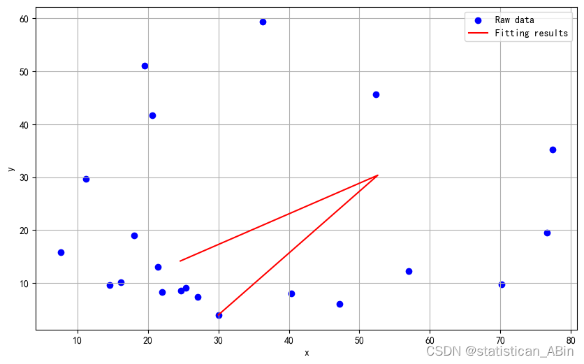
Fitting parameter values:a=-0.04946907994199101, b=5.5137169943224755, c=0.6909170053541569, d=10.615879287885402, e=-3.1585499451409937, f=18.4110095977882
发现效果竟然变差了
#Set parameter search range (interval)
bounds = [(-0.1, 10), (-0.1, 10), (-0.1, 10), (-0.1,10), (-0.1, 10), (-0.1, 10)]
# Use interval search to set initial parameter values
result = differential_evolution(error, bounds)
a_fit, b_fit, c_fit, d_fit, e_fit, f_fit = result.x
# Simulate the fitted trajectory
t_fit = np.linspace(0, 1, len(data))
y0_fit = [data[0, 0], data[0, 1]]
y_fit = odeint(model, y0_fit, t_fit, args=(a_fit, b_fit, c_fit, d_fit, e_fit, f_fit))
x_fit, z_fit = y_fit[:, 0], y_fit[:, 1]
# Plot the fitting results against the original data points
plt.figure(figsize=(10, 6))
plt.scatter(data[:, 0], data[:, 1], label='Raw data', marker='o', color='blue')
plt.plot(x_fit, z_fit, label='Fitting results', linestyle='-', color='red')
plt.xlabel('x')
plt.ylabel('y')
plt.legend()
plt.grid()
plt.show()
print(f"Fitting parameter values:a={a_fit}, b={b_fit}, c={c_fit}, d={d_fit}, e={e_fit}, f={f_fit}")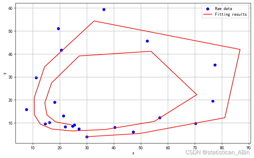 最终优化结果为:
Fitting parameter values:a=10.0, b=0.6320729493793303, c=10.0, d=0.4325244090515547, e=-0.07495645186059174, f=0.18793803443302332
创作不易,希望大家多点赞关注评论!!!