引言
旋转位置编码(Rotary Position Embedding, RoPE)将绝对相对位置依赖纳入自注意力机制中,以增强Transformer架构的性能。目前很火的大模型LLaMA、QWen等都应用了旋转位置编码。
之前在[论文笔记]ROFORMER中对旋转位置编码的原始论文进行了解析,重点推导了旋转位置编码的公式,本文侧重实现,同时尽量简化数学上的推理,详细推理可见最后的参考文章。
复数与极坐标
复数由两个部分组成:实部(real part)和虚部(imaginary part)。实部就是一个普通的数字,可以是零、正数或负数。虚部是另一个实数与 i i i相乘。比如 2 + 3 i 2+3i 2+3i是一个复数,其中 2 2 2是实部; 3 i 3i 3i是虚部。下面这些数字都是复数:
2 , 2 + 2 i , 1 − 3 i , − 4 i , 17 i 2, \quad 2+2i,\quad 1-3i,\quad -4i,\quad 17i 2,2+2i,1−3i,−4i,17i
可以看到复数是实数的扩展,包含了实数,比如 2 2 2可以看成是虚部为 0 0 0。
通常实数放前面,然后是 i i i。但当 i i i与三角函数( sin , cos \sin,\cos sin,cos)在一起通常把 i i i放在前面: i sin θ , i cos θ i \sin \theta, i\cos \theta isinθ,icosθ。
i i i我们可以理解为就是一个简单的数学对象,满足 i 2 = − 1 i^2=-1 i2=−1。
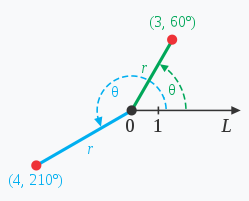
极坐标系是一个二维坐标系统。该坐标系统中任意位置可由一个夹角和一段相对原点——极点的距离来表示。如上图(来自百度百科)所示。
给定极坐标系内的任意一个复数 x + y i x+yi x+yi(对应二维向量 [ x , y ] [x,y] [x,y]),要将其(逆时针)旋转 θ \theta θ度,只需要乘上旋转子:
R θ = cos θ + i sin θ ( sin 2 θ + cos 2 θ = 1 ) (1) \pmb R_\theta = \cos \theta + i \sin \theta \qquad(\sin^2 \theta + \cos^2 \theta = 1) \tag 1 Rθ=cosθ+isinθ(sin2θ+cos2θ=1)(1)
可以相乘再展开,然后利用 i 2 = − 1 i^2=-1 i2=−1可得:
x ′ + y ′ i = ( cos θ + i sin θ ) ( x + y i ) = ( x cos θ − y sin θ ) + ( x sin θ + y cos θ ) i \begin{aligned} x^\prime + y^\prime i &= (\cos \theta + i\sin \theta)(x + yi) \\ &= (x \cos \theta - y \sin \theta)+(x \sin \theta + y \cos \theta)i \end{aligned} x′+y′i=(cosθ+isinθ)(x+yi)=(xcosθ−ysinθ)+(xsinθ+ycosθ)i
对应二维平面中点 [ x , y ] [x,y] [x,y]关于原点的逆时针旋转:
[ x ′ y ′ ] = [ cos θ − sin θ sin θ cos θ ] [ x y ] \begin{bmatrix} x^\prime \\ y^\prime \end{bmatrix} = \begin{bmatrix} \cos \theta & -\sin \theta \\ \sin \theta & \cos \theta \end{bmatrix} \begin{bmatrix} x \\ y \end{bmatrix} [x′y′]=[cosθsinθ−sinθcosθ][xy]
其中包含 θ \theta θ的矩阵是一个旋转矩阵。
旋转位置编码
x i ∈ R d \pmb x_i \in \Bbb R^d xi∈Rd是无位置信息的标记 w i w_i wi的 d d d维词嵌入向量。自注意力首先将位置信息与单词嵌入相结合,并将其转化为query、key和value的表示形式。
q m = f q ( x m , m ) k n = f k ( x n , n ) v n = f v ( x n , n ) (2) \begin{aligned} \pmb q_m &= f_q(\pmb x_m, m) \\ \pmb k_n &= f_k(\pmb x_n, n) \\ \pmb v_n &= f_v(\pmb x_n, n) \\ \end{aligned} \tag 2 qmknvn=fq(xm,m)=fk(xn,n)=fv(xn,n)(2)
其中 q m , k n \pmb q_m,\pmb k_n qm,kn和 v n \pmb v_n vn分别通过 f q , f k f_q,f_k fq,fk和 f v f_v fv整合了第m和第n个位置信息。query和key然后用于计算注意力权重,而输出为value的加权和。
a m , n = exp ( q m T k n d ) ∑ j = 1 N exp q m T k j d o m = ∑ n = 1 N a m , n v n (3) \begin{aligned} a_{m,n} &= \frac{\exp(\frac{\pmb q^T_m \pmb k_n}{\sqrt d})}{\sum_{j=1}^N \exp \frac{\pmb q^T_m \pmb k_j}{\sqrt d}} \\ \pmb o_m &= \sum_{n=1}^N a_{m,n}\pmb v_n \\ \end{aligned} \tag 3 am,nom=∑j=1NexpdqmTkjexp(dqmTkn)=n=1∑Nam,nvn(3)
Transformer通过自注意机制利用各个标记的位置信息,如等式(3)中所见, q m T k n \pmb q_m^T \pmb k_n qmTkn通常可以在不同位置的标记之间传递知识。为了融入相对位置信息,我们需要将查询 q m \pmb q_m qm和键 k n \pmb k_n kn的内积公式转化为一个函数 g g g,该函数只接受词嵌入 x m , x n \pmb x_m,\pmb x_n xm,xn以及它们的相对位置 m − n m-n m−n作为输入变量。换句话说,我们希望内积只以相对形式编码位置信息:
⟨ f q ( x m , m ) , f k ( x n , n ) ⟩ = g ( x m , x n , m − n ) (4) \langle f_q(\pmb x_m,m) , f_k(\pmb x_n,n) \rangle = g(\pmb x_m,\pmb x_n, m-n) \tag 4 ⟨fq(xm,m),fk(xn,n)⟩=g(xm,xn,m−n)(4)
最终目标是找到一个等价的编码方式来求解函数 f q ( x m , m ) f_q(\pmb x_m, m) fq(xm,m)和 f k ( x n , n ) f_k(\pmb x_n, n) fk(xn,n),以符合上等式。
从简单的维度 d = 2 d=2 d=2的情况开始,这样可以利用二维平面上向量的几何特性及其复数形式来证明公式(4)的一个解是:
f q ( x m , m ) = ( W q x m ) e i m θ f k ( x n , n ) = ( W k x n ) e i n θ g ( x m , x n , m − n ) = Re [ ( W q x m ) ( W k x n ) ∗ e i ( m − n ) θ ] (5) \begin{aligned} f_q(\pmb x_m,m) &= (\pmb W_q\pmb x_m) e^{im\theta} \\ f_k(\pmb x_n,n) &= (\pmb W_k\pmb x_n) e^{in\theta} \\ g(\pmb x_m,\pmb x_n,m-n) &= \text{Re}[(\pmb W_q\pmb x_m)(\pmb W_k\pmb x_n)^*e^{i(m-n)\theta}] \end{aligned} \tag {5} fq(xm,m)fk(xn,n)g(xm,xn,m−n)=(Wqxm)eimθ=(Wkxn)einθ=Re[(Wqxm)(Wkxn)∗ei(m−n)θ](5)
这里 Re [ ⋅ ] \text{Re}[\cdot] Re[⋅]表示复数的实部; ( W k x n ) ∗ (\pmb W_k\pmb x_n)^* (Wkxn)∗表示 ( W k x n ) (\pmb W_k\pmb x_n) (Wkxn)的共轭复数; θ ∈ R \theta \in \Bbb R θ∈R表示一个非零常数。
可以进一步将 f { q , k } f_{\{q,k\}} f{q,k}写成矩阵乘法形式:
f { q , k } ( x m , m ) = ( cos m θ − sin m θ sin m θ cos m θ ) ( W { q , k } ( 11 ) W { q , k } ( 12 ) W { q , k } ( 21 ) W { q , k } ( 22 ) ) ( x m ( 1 ) x m ( 2 ) ) (6) f_{\{q,k\}} (\pmb x_m,m) =\begin{pmatrix} \cos m\theta & -\sin m\theta \\ \sin m\theta & \cos m\theta \end{pmatrix}\begin{pmatrix} W_{\{q,k\}}^{(11)} & W_{\{q,k\}}^{(12)} \\ W_{\{q,k\}}^{(21)} & W_{\{q,k\}}^{(22)} \end{pmatrix} \begin{pmatrix} x_m^{(1)} \\ x_m^{(2)} \end{pmatrix} \tag{6} f{q,k}(xm,m)=(cosmθsinmθ−sinmθcosmθ)(W{q,k}(11)W{q,k}(21)W{q,k}(12)W{q,k}(22))(xm(1)xm(2))(6)
这里的 { q , k } \{q,k\} {q,k}表示 q q q和 k k k的集合,比如上式对 f q f_q fq和 f k f_k fk都成立;包含 sin m θ \sin m\theta sinmθ或 cos m θ \cos m\theta cosmθ的矩阵是上面介绍的旋转矩阵。
其中$ (x^{(1)}_m, x^{(2)}_m) 为 为 为x_m$ 在二维坐标中的表示。类似地, g g g 可以被视为一个矩阵,从而能够在二维情况下求解等式 ( 4 ) (4) (4)。具体来说,结合相对位置嵌入是很直接的:只需将仿射变换后的词嵌入向量旋转一定角度乘位置索引(旋转 m θ m\theta mθ),从而解释了旋转位置嵌入背后的直觉。
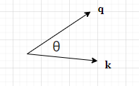
我们进行直观理解,假设两个向量 q \pmb q q和 k \pmb k k它们的夹角为 θ \theta θ,根据向量夹角的余弦我们知道 q ⋅ k = ∣ q ∣ ∣ k ∣ cos θ \pmb q \cdot \pmb k = |\pmb q||\pmb k| \cos \theta q⋅k=∣q∣∣k∣cosθ。
当 q \pmb q q(逆时针)旋转 α \alpha α角度后,与 k \pmb k k的夹角变成了 θ + α \theta + \alpha θ+α:

当 k \pmb k k旋转 β \beta β角度后,与 q \pmb q q的夹角变成了 θ − β \theta - \beta θ−β:
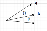
当两个向量同时旋转后,它们的夹角变成了 θ + α − β \theta + \alpha -\beta θ+α−β。内积表达式为:
q ⋅ k = ∣ q ∣ ∣ k ∣ cos ( θ + α − β ) \pmb q \cdot \pmb k = |\pmb q||\pmb k| \cos (\theta + \alpha - \beta) q⋅k=∣q∣∣k∣cos(θ+α−β)
特殊地,当 α − β = 0 \alpha - \beta =0 α−β=0时,即两个向量旋转的角度相同,它们的内积不变。通过这两个向量的夹角来影响内积的值。通过这种直觉,公式(4)是成立的。
为了将我们在二维空间中的结果推广到任意 x i ∈ R d \pmb x_i ∈ \R^d xi∈Rd,其中 d d d 是偶数。我们可以将 d d d 维空间划分为 $d/2 $个子空间(分块矩阵),并结合内积的线性特性进行组合,将 f { q , k } f_{\{q,k\}} f{q,k} 转化为:
f { q , k } = ( x m , m ) = R Θ , m d W { q , k } x m (7) f_{\{q,k\}} = (\pmb x_m,m) = \pmb R_{\Theta,m}^d \pmb W_{\{q,k\}} \pmb x_m \tag{7} f{q,k}=(xm,m)=RΘ,mdW{q,k}xm(7)
这里说的特性是指线性叠加性:
定义:内积的定义是两个向量对应分量相乘后再相加。假设有两个向量 v ⃗ = ( v 1 , v 2 , . . . , v n ) \vec{v} = (v_1, v_2, ..., v_n) v=(v1,v2,...,vn) 和 w ⃗ = ( w 1 , w 2 , . . . , w n ) \vec{w} = (w_1, w_2, ..., w_n) w=(w1,w2,...,wn),它们的内积可以表示为 v ⃗ ⋅ w ⃗ = v 1 w 1 + v 2 w 2 + . . . + v n w n \vec{v} \cdot \vec{w} = v_1w_1 + v_2w_2 + ... + v_nw_n v⋅w=v1w1+v2w2+...+vnwn。
线性性质:内积满足线性叠加性,即对于任意标量 a a a 和向量 v ⃗ , w ⃗ , u ⃗ \vec{v}, \vec{w}, \vec{u} v,w,u,有以下性质:
- 可加性: v ⃗ ⋅ ( w ⃗ + u ⃗ ) = v ⃗ ⋅ w ⃗ + v ⃗ ⋅ u ⃗ \vec{v} \cdot (\vec{w} + \vec{u}) = \vec{v} \cdot \vec{w} + \vec{v} \cdot \vec{u} v⋅(w+u)=v⋅w+v⋅u
- 齐次性: ( a v ⃗ ) ⋅ w ⃗ = a ( v ⃗ ⋅ w ⃗ ) (a\vec{v}) \cdot \vec{w} = a(\vec{v} \cdot \vec{w}) (av)⋅w=a(v⋅w)
其中
R Θ , m d = ( cos m θ 1 − sin m θ 1 0 0 ⋯ 0 0 sin m θ 1 cos m θ 1 0 0 ⋯ 0 0 0 0 cos m θ 2 − sin m θ 2 ⋯ 0 0 0 0 sin m θ 2 cos m θ 2 ⋯ 0 0 ⋮ ⋮ ⋮ ⋮ ⋱ ⋮ ⋮ 0 0 0 0 ⋯ cos m θ d / 2 − sin m θ d / 2 0 0 0 0 ⋯ sin m θ d / 2 cos m θ d / 2 ) (8) \pmb R_{\Theta,m}^d = \begin{pmatrix} \cos m\theta_1 & -\sin m\theta_1 & 0 & 0 & \cdots & 0 & 0 \\ \sin m\theta_1 & \cos m\theta_1 & 0 & 0 & \cdots & 0 & 0 \\ 0 & 0 & \cos m\theta_2 & -\sin m\theta_2 & \cdots & 0 & 0 \\ 0 & 0 & \sin m\theta_2 & \cos m\theta_2 & \cdots & 0 & 0 \\ \vdots & \vdots & \vdots & \vdots & \ddots & \vdots & \vdots \\ 0 & 0 & 0 & 0 & \cdots & \cos m\theta_{d/2} & -\sin m\theta_{d/2} \\ 0 & 0 & 0 & 0 & \cdots & \sin m\theta_{d/2} & \cos m\theta_{d/2} \\ \end{pmatrix} \tag{8} RΘ,md=
cosmθ1sinmθ100⋮00−sinmθ1cosmθ100⋮0000cosmθ2sinmθ2⋮0000−sinmθ2cosmθ2⋮00⋯⋯⋯⋯⋱⋯⋯0000⋮cosmθd/2sinmθd/20000⋮−sinmθd/2cosmθd/2
(8)
是一个带有预定义参数 Θ = { θ i = 1000 0 − 2 ( i − 1 ) / d , i ∈ [ 1 , 2 , . . . , d / 2 ] } Θ = \{θ_i = 10000^{−2(i−1)/d}, i ∈ [1, 2, ..., d/2]\} Θ={θi=10000−2(i−1)/d,i∈[1,2,...,d/2]} 的旋转矩阵。RoPE的图示如原论文中的图(1)所示。将RoPE应用于等式(3)中的自注意力机制,我们可以得到:
q m ⊤ k n = ( R Θ , m d W q x m ) ⊤ ( R Θ , n d W k x n ) = x m ⊤ W q R Θ , n − m d W k x n (9) \pmb q_m^\top \pmb k_n = (\pmb R_{\Theta,m}^d \pmb W_{q}\pmb x_m)^\top (\pmb R_{\Theta,n}^d \pmb W_{k}\pmb x_n) = \pmb x_m^\top \pmb W_q \pmb R_{\Theta,n-m}^d \pmb W_k \pmb x_n \tag{9} qm⊤kn=(RΘ,mdWqxm)⊤(RΘ,ndWkxn)=xm⊤WqRΘ,n−mdWkxn(9)
其中 R Θ , n − m d = ( R Θ , m d ) ⊤ R Θ , n d \pmb R_{\Theta,n-m}^d=(\pmb R_{\Theta,m}^d)^\top \pmb R_{\Theta,n}^d RΘ,n−md=(RΘ,md)⊤RΘ,nd。值得指出的是, R Θ \pmb R_{\Theta} RΘ是一个正交矩阵,它不会改变向量的模长,因此通常来说它不会改变原模型的稳定性。
我们可以增大 θ \theta θ的base以支持更长的上下文,这里是10000。
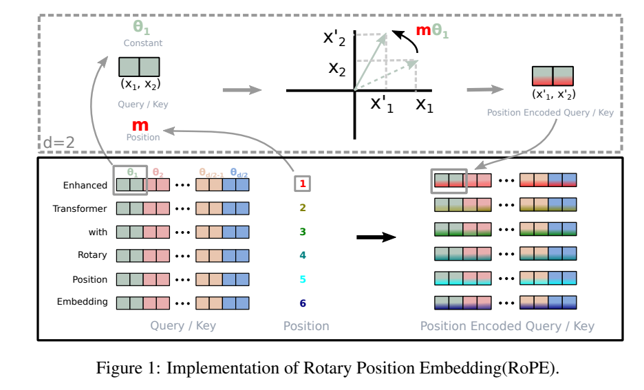
上图所说的是一个长度为6的序列,在进行自注意力计算时,Query和Key向量经过旋转位置编码变换的过程。首先对于位置1来说,记为 m m m。然后仅考虑第一个二维子空间,即 ( x 1 , x 2 ) (x_1,x_2) (x1,x2)向量,旋转 m θ 1 m\theta_1 mθ1后得到的增强表示。
由于公式(8)中 R Θ , m d \pmb R^d_{\Theta,m} RΘ,md的稀疏性,可以通过下述等价方式来实现 R Θ , m d \pmb R^d_{\Theta,m} RΘ,md和 x ∈ R d \pmb x \in \R^d x∈Rd的乘法:
R Θ , m d x = ( x 1 x 2 x 3 x 4 ⋮ x d − 1 x d ) ⊗ ( cos m θ 1 cos m θ 1 cos m θ 2 cos m θ 2 ⋮ cos m θ d / 2 cos m θ d / 2 ) + ( − x 2 x 1 − x 4 x 3 ⋮ − x d x d − 1 ) ⊗ ( sin m θ 1 sin m θ 1 sin m θ 2 sin m θ 2 ⋮ sin m θ d / 2 sin m θ d / 2 ) (10) \pmb R^d_{\Theta,m} \pmb x =\begin{pmatrix}x_1 \\ x_2 \\ x_3 \\ x_4 \\ \vdots \\ x_{d-1} \\ x_{d} \end{pmatrix}\otimes\begin{pmatrix}\cos m\theta_1 \\ \cos m\theta_1 \\ \cos m\theta_2 \\ \cos m\theta_2 \\ \vdots \\ \cos m\theta_{d/2} \\ \cos m\theta_{d/2} \end{pmatrix} + \begin{pmatrix}-x_2 \\ x_1 \\ -x_4 \\ x_3 \\ \vdots \\ -x_{d} \\ x_{d-1} \end{pmatrix}\otimes\begin{pmatrix}\sin m\theta_1 \\ \sin m\theta_1 \\ \sin m\theta_2 \\ \sin m\theta_2 \\ \vdots \\ \sin m\theta_{d/2} \\ \sin m\theta_{d/2} \end{pmatrix} \tag{10} RΘ,mdx=
x1x2x3x4⋮xd−1xd
⊗
cosmθ1cosmθ1cosmθ2cosmθ2⋮cosmθd/2cosmθd/2
+
−x2x1−x4x3⋮−xdxd−1
⊗
sinmθ1sinmθ1sinmθ2sinmθ2⋮sinmθd/2sinmθd/2
(10)
其中 ⊗ \otimes ⊗是逐位对应相乘。
为什么可以简化成这样子,把乘 x \pmb x x带入公式(8)得到:
R Θ , m d x = ( cos m θ 1 − sin m θ 1 0 0 ⋯ 0 0 sin m θ 1 cos m θ 1 0 0 ⋯ 0 0 0 0 cos m θ 2 − sin m θ 2 ⋯ 0 0 0 0 sin m θ 2 cos m θ 2 ⋯ 0 0 ⋮ ⋮ ⋮ ⋮ ⋱ ⋮ ⋮ 0 0 0 0 ⋯ cos m θ d / 2 − sin m θ d / 2 0 0 0 0 ⋯ sin m θ d / 2 cos m θ d / 2 ) ( x 1 x 2 x 3 x 4 ⋮ x d − 1 x d ) \pmb R_{\Theta,m}^d \pmb x= \begin{pmatrix}\begin{array}{cc:cc:cc:cc} \cos m\theta_1 & -\sin m\theta_1 & 0 & 0 & \cdots & 0 & 0 \\ \sin m\theta_1 & \cos m\theta_1 & 0 & 0 & \cdots & 0 & 0 \\ \hdashline 0 & 0 & \cos m\theta_2 & -\sin m\theta_2 & \cdots & 0 & 0 \\ 0 & 0 & \sin m\theta_2 & \cos m\theta_2 & \cdots & 0 & 0 \\ \hdashline \vdots & \vdots & \vdots & \vdots & \ddots & \vdots & \vdots \\ \hdashline 0 & 0 & 0 & 0 & \cdots & \cos m\theta_{d/2} & -\sin m\theta_{d/2} \\ 0 & 0 & 0 & 0 & \cdots & \sin m\theta_{d/2} & \cos m\theta_{d/2} \\ \end{array}\end{pmatrix} \begin{pmatrix}x_1 \\ x_2 \\ \hdashline x_3 \\ x_4 \\ \hdashline\vdots \\ \hdashline x_{d-1} \\ x_{d}\end{pmatrix} RΘ,mdx=
cosmθ1sinmθ100⋮00−sinmθ1cosmθ100⋮0000cosmθ2sinmθ2⋮0000−sinmθ2cosmθ2⋮00⋯⋯⋯⋯⋱⋯⋯0000⋮cosmθd/2sinmθd/20000⋮−sinmθd/2cosmθd/2
x1x2x3x4⋮xd−1xd
根据分块矩阵的乘法,我们仅考虑左右两边矩阵的第一块,其得到(10)中向量的第1和第2个元素:
( cos m θ 1 − sin m θ 1 sin m θ 1 cos m θ 1 ) ( x 1 x 2 ) = ( x 1 cos m θ 1 − x 2 sin m θ 1 x 1 sin m θ 1 + x 2 cos m θ 1 ) \begin{pmatrix} \cos m\theta_1 & -\sin m\theta_1\\ \sin m\theta_1 & \cos m\theta_1 \end{pmatrix} \begin{pmatrix} x_1\\ x_2 \end{pmatrix} = \begin{pmatrix}x_1 \cos m\theta_1 - x_2 \sin m\theta_1 \\ x_1 \sin m\theta_1+x_2 \cos m\theta_1 \end{pmatrix} (cosmθ1sinmθ1−sinmθ1cosmθ1)(x1x2)=(x1cosmθ1−x2sinmθ1x1sinmθ1+x2cosmθ1)
因此这是成立的。
代码实现
本节参考LLaMA源码来实现旋转位置编码,同时底层实现逻辑进行一个解释。
首先定义一个函数生成旋转矩阵:
def precompute_freqs_cis(dim: int, end: int, theta: float = 10000.0):
  """
  给定维度预计算频率(\theta) Tensor的复指数(complex exponentials,cis)
  Args:
    dim (int): dimension of the frequency tensor
    end (int): end index for precomputing frequencies
    theta (float, optional): scaling factor for frequency computation. Defaults to 10000.0.

  Returns:
    torch.Tensor: Precomputed frequency tensor with complex exponentials.
  """
  # freqs (dim/2, )
  # theta_i = 10000 ** (-2(i-1)/dim) for i = [1,2,...,dim / 2]
  # theta_i
  # we start from 0 dont need to do i-1
  freqs = 1.0 / (theta ** (torch.arange(0, dim, 2).float() / dim))
  # generate token sequence m = [0, 1, ..., seq_len - 1]
  # m (end, )
  m = torch.arange(end, device=freqs.device)
  # compute m * \theta
  # freqs (end, dim / 2)
  freqs = torch.outer(m, freqs).float()
  # freqs_cis (end, dim / 2)
  freqs_cis = torch.polar(torch.ones_like(freqs), freqs)
  return freqs_cis
这个函数用于生成公式(8)中的旋转矩阵。
首先计算预定义参数 Θ = { θ i = 1000 0 − 2 ( i − 1 ) / d , i ∈ [ 1 , 2 , . . . , d / 2 ] } Θ = \{θ_i = 10000^{−2(i−1)/d}, i ∈ [1, 2, ..., d/2]\} Θ={θi=10000−2(i−1)/d,i∈[1,2,...,d/2]} ,我们的 i i i从 0 0 0开始因此不需要 i − 1 i-1 i−1,对应上面的Line 17。
然后考虑所有的位置,生成一个m = (seq_len, )形状的向量,Line 20。
计算m和Line 17计算出来的freqs的外积,即m中的每个位置 m i m_i mi都会乘上 Θ Θ Θ的每个元素,得到一个(seq_len, dim / 2)形状的矩阵。假设序列的长度
假设 m = [ m 1 , m 2 , ⋯ , m T ] = [ 1 , 2 , ⋯ , N ] m=[m_1,m_2,\cdots,m_T] =[1,2,\cdots, N] m=[m1,m2,⋯,mT]=[1,2,⋯,N],这里 N N N表示序列长度。
它们的乘积是一个矩阵:
( m 1 θ 1 m 1 θ 2 ⋯ m 1 θ d / 2 m 2 θ 1 m 2 θ 2 ⋯ m 2 θ d / 2 ⋮ ⋮ ⋱ ⋮ m N θ 1 m N θ 2 ⋯ m N θ d / 2 ) \begin{pmatrix} m_1 \theta_1 & m_1 \theta_2 & \cdots & m_1 \theta_{d/2} \\ m_2 \theta_1 & m_2 \theta_2 & \cdots & m_2 \theta_{d/2} \\ \vdots & \vdots &\ddots &\vdots \\ m_N \theta_1 & m_N \theta_2 & \cdots & m_N \theta_{d/2} \end{pmatrix}
m1θ1m2θ1⋮mNθ1m1θ2m2θ2⋮mNθ2⋯⋯⋱⋯m1θd/2m2θd/2⋮mNθd/2
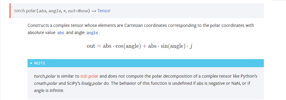
最后在Line 25通过 torch.polar将它们转换为复数形式:
( cos ( m 1 θ 1 ) + i ⋅ sin ( m 1 θ 1 ) cos ( m 1 θ 2 ) + i ⋅ sin ( m 1 θ 2 ) ⋯ cos ( m 1 θ d / 2 ) + i ⋅ sin ( m 1 θ d / 2 ) cos ( m 2 θ 1 ) + i ⋅ sin ( m 2 θ 1 ) cos ( m 2 θ 2 ) + i ⋅ sin ( m 2 θ 2 ) ⋯ cos ( m 2 θ d / 2 ) + i ⋅ sin ( m 2 θ d / 2 ) ⋮ ⋮ ⋱ ⋮ cos ( m N θ 1 ) + i ⋅ sin ( m N θ 1 ) cos ( m N θ 2 ) + i ⋅ sin ( m N θ 2 ) ⋯ cos ( m N θ d / 2 ) + i ⋅ sin ( m N θ d / 2 ) ) \begin{pmatrix} \cos(m_1 \theta_1) + i\cdot \sin(m_1 \theta_1) & \cos(m_1 \theta_2) + i\cdot \sin(m_1 \theta_2) & \cdots & \cos(m_1 \theta_{d/2}) + i\cdot \sin(m_1 \theta_{d/2}) \\ \cos(m_2 \theta_1) + i\cdot \sin(m_2 \theta_1) & \cos(m_2 \theta_2) + i\cdot \sin(m_2 \theta_2) & \cdots & \cos(m_2 \theta_{d/2}) + i\cdot \sin(m_2 \theta_{d/2}) \\ \vdots & \vdots &\ddots &\vdots \\ \cos(m_N \theta_1) + i\cdot \sin(m_N \theta_1) & \cos(m_N \theta_2) + i\cdot \sin(m_N \theta_2) & \cdots & \cos(m_N \theta_{d/2}) + i\cdot \sin(m_N \theta_{d/2}) \\ \end{pmatrix}
cos(m1θ1)+i⋅sin(m1θ1)cos(m2θ1)+i⋅sin(m2θ1)⋮cos(mNθ1)+i⋅sin(mNθ1)cos(m1θ2)+i⋅sin(m1θ2)cos(m2θ2)+i⋅sin(m2θ2)⋮cos(mNθ2)+i⋅sin(mNθ2)⋯⋯⋱⋯cos(m1θd/2)+i⋅sin(m1θd/2)cos(m2θd/2)+i⋅sin(m2θd/2)⋮cos(mNθd/2)+i⋅sin(mNθd/2)
torch.polar(abs, angle)基于abs和angle计算出一个极坐标系中的复数表示:
那如何达到公式(10)的结果呢,为了简单,这里只展示 d = 4 d=4 d=4的情况,考虑某个Token x \pmb x x:
x = [ x 1 x 2 x 3 x 4 ] \pmb x=\begin{bmatrix} x_1 & x_2 & x_3 & x_4 \end{bmatrix} x=[x1x2x3x4]
第一步把 x \pmb x x的元素两两分组:
x = [ [ x 1 , x 2 ] [ x 3 , x 4 ] ] \pmb x=\begin{bmatrix} [x_1 ,x_2 ] & [x_3 ,x_4] \end{bmatrix} x=[[x1,x2][x3,x4]]
也不考虑批次维度,形状由(1,4)变成(1,2,2)。然后把新的 x \pmb x x转换成复数的形式,形状变成了(1, 2):
x = [ x 1 + i ⋅ x 2 x 3 + i ⋅ x 4 ] \pmb x=\begin{bmatrix} x_1 + i\cdot x_2 & x_3 + i \cdot x_4 \end{bmatrix} x=[x1+i⋅x2x3+i⋅x4]
即每个二维向量变成了一个复数。然后我们把这个向量矩阵和freqs_cis对应的向量对应位置相乘(分别旋转 m θ 1 , m θ 2 m\theta_1,m\theta_2 mθ1,mθ2角度: d / 2 = 4 / 2 = 2 d/2=4/2=2 d/2=4/2=2),这里假设当前位置为 m m m,然后有:
x = [ x 1 + i ⋅ x 2 x 3 + i ⋅ x 4 ] ⊗ [ cos ( m θ 1 ) + i ⋅ sin ( m θ 1 ) cos ( m θ 2 ) + i ⋅ sin ( m θ 2 ) ] = [ ( x 1 + i ⋅ x 2 ) [ cos ( m θ 1 ) + i ⋅ sin ( m θ 1 ) ] ( x 3 + i ⋅ x 4 ) [ cos ( m θ 2 ) + i ⋅ sin ( m θ 2 ) ] ] = [ x 1 cos m θ 1 + i ⋅ x 1 sin m θ 1 + i ⋅ x 2 cos m θ 1 − x 2 sin m θ 1 x 3 cos m θ 2 + i ⋅ x 3 sin m θ 2 + i ⋅ x 4 cos m θ 2 − x 4 sin m θ 2 ] = [ x 1 cos m θ 1 − x 2 sin m θ 1 + i ( x 1 sin m θ 1 + x 2 cos m θ 1 ) x 3 cos m θ 2 − x 4 sin m θ 2 + i ( x 3 sin m θ 2 + x 4 cos m θ 2 ) ] \begin{aligned} \pmb x &=\begin{bmatrix} x_1 + i\cdot x_2 & x_3 + i \cdot x_4 \end{bmatrix} \otimes \begin{bmatrix} \cos(m \theta_1) + i\cdot \sin(m \theta_1) & \cos(m \theta_2) + i\cdot \sin(m \theta_2)\end{bmatrix} \\ &= \begin{bmatrix} (x_1 + i\cdot x_2) [\cos(m \theta_1) + i\cdot \sin(m \theta_1)] & (x_3 + i \cdot x_4) [\cos(m \theta_2) + i\cdot \sin(m \theta_2)] \end{bmatrix} \\ &= \begin{bmatrix} x_1 \cos m \theta_1 +i\cdot x_1 \sin m \theta_1 + i \cdot x_2 \cos m \theta_1 - x_2 \sin m \theta_1 & x_3 \cos m \theta_2 +i\cdot x_3 \sin m \theta_2 + i \cdot x_4 \cos m \theta_2 - x_4 \sin m \theta_2 \end{bmatrix} \\ &= \begin{bmatrix} x_1 \cos m \theta_1 - x_2 \sin m \theta_1+ i(x_1 \sin m \theta_1 + x_2 \cos m \theta_1) & x_3 \cos m \theta_2 -x_4 \sin m \theta_2 +i(x_3 \sin m \theta_2 +x_4 \cos m \theta_2) \end{bmatrix} \\ \end{aligned} x=[x1+i⋅x2x3+i⋅x4]⊗[cos(mθ1)+i⋅sin(mθ1)cos(mθ2)+i⋅sin(mθ2)]=[(x1+i⋅x2)[cos(mθ1)+i⋅sin(mθ1)](x3+i⋅x4)[cos(mθ2)+i⋅sin(mθ2)]]=[x1cosmθ1+i⋅x1sinmθ1+i⋅x2cosmθ1−x2sinmθ1x3cosmθ2+i⋅x3sinmθ2+i⋅x4cosmθ2−x4sinmθ2]=[x1cosmθ1−x2sinmθ1+i(x1sinmθ1+x2cosmθ1)x3cosmθ2−x4sinmθ2+i(x3sinmθ2+x4cosmθ2)]
得到一个形状为(1,2)的复数项链。
然后我们把里面的复数变为二维向量:
x = [ [ x 1 cos m 1 θ 1 − x 2 sin m 1 θ 1 x 1 sin m 1 θ 1 + x 2 cos m 1 θ 1 ] [ x 3 cos m 1 θ 2 − x 4 sin m 1 θ 2 x 3 sin m 1 θ 2 + x 4 cos m 1 θ 2 ] ] \pmb x= \begin{bmatrix} \begin{bmatrix} x_1 \cos m_1 \theta_1 - x_2 \sin m_1 \theta_1 \\ x_1 \sin m_1 \theta_1 + x_2 \cos m_1 \theta_1 \end{bmatrix} & \begin{bmatrix} x_3 \cos m_1 \theta_2 -x_4 \sin m_1 \theta_2 \\ x_3 \sin m_1 \theta_2 +x_4 \cos m_1 \theta_2 \end{bmatrix} \end{bmatrix} x=[[x1cosm1θ1−x2sinm1θ1x1sinm1θ1+x2cosm1θ1][x3cosm1θ2−x4sinm1θ2x3sinm1θ2+x4cosm1θ2]]
最后拉平其中的二维向量:
x = [ x 1 cos m θ 1 − x 2 sin m θ 1 x 1 sin m θ 1 + x 2 cos m θ 1 x 3 cos m θ 2 − x 4 sin m θ 2 x 3 sin m θ 2 + x 4 cos m 1 θ 2 ] \pmb x= \begin{bmatrix} x_1 \cos m \theta_1 - x_2 \sin m \theta_1 & x_1 \sin m \theta_1 + x_2 \cos m \theta_1 & x_3 \cos m \theta_2 -x_4 \sin m \theta_2 & x_3 \sin m \theta_2 +x_4 \cos m_1 \theta_2 \end{bmatrix} x=[x1cosmθ1−x2sinmθ1x1sinmθ1+x2cosmθ1x3cosmθ2−x4sinmθ2x3sinmθ2+x4cosm1θ2]
比较公式(10)中前4行的结果,可以发现是一样的,只不过列向量变成了行向量。
基于上面的过程我们就不难理解下面的代码:
def apply_rotary_emb(xq: Tensor, xk: Tensor, freq_cis: Tensor):
  """

  使用给定的频率Tensor将旋转嵌入应用到输入张量中。

  该函数使用提供的频率使用给定的频率Tensor将旋转嵌入应用到输入张量中。
  freqs_cis将旋转嵌入应用到给定的查询xq和键xk张量上。输入张量被重塑为复数,并且频率张量被重塑以匹配广播兼容性。生成的张量包含旋转嵌入,并作为实张量返回。

  Args:
      xq (torch.Tensor): Query tensor to apply rotary embeddings.
      xk (torch.Tensor): Key tensor to apply rotary embeddings.
      freqs_cis (torch.Tensor): Precomputed frequency tensor for complex exponentials.

  Returns:
      Tuple[torch.Tensor, torch.Tensor]: Tuple of modified query tensor and key tensor with rotary embeddings.

  """
  # xq (batch_size, seq_len, n_head, head_dim)
  # xq_ (batch_size, seq_len, n_head, head_dim // 2, 2)
  xq_ = xq.float().reshape(*xq.shape[:-1], -1, 2)
  xk_ = xk.float().reshape(*xk.shape[:-1], -1, 2)

  # turn to complex
  # xq_ (batch_size, seq_len, n_head, head_dim // 2)
  xq_ = torch.view_as_complex(xq_)
  xk_ = torch.view_as_complex(xk_)

  # 应用旋转操作,然后将结果转回实数
  # xq_out (batch_size, seq_len, n_head, head_dim)
  xq_out = torch.view_as_real(xq_ * freq_cis).flatten(2)
  xk_out = torch.view_as_real(xk_ * freq_cis).flatten(2)

  return xq_out.type_as(xq), xk_out.type_as(xk)
下篇文章我们会探讨如何应用旋转位置编码到自注意力上。