目录
政安晨的个人主页:政安晨
欢迎 👍点赞✍评论⭐收藏
收录专栏: TensorFlow与Keras机器学习实战
希望政安晨的博客能够对您有所裨益,如有不足之处,欢迎在评论区提出指正!
文本目标:在 UCF101 数据集上使用迁移学习和递归模型训练视频分类器。
该示例演示了视频分类,这是在推荐、安全等领域应用的一个重要用例。
我们将使用 UCF101 数据集来构建视频分类器。
该数据集包含按不同动作分类的视频,如板球投篮、拳击、骑自行车等。
该数据集通常用于构建动作识别器,这是视频分类的一种应用。
视频由有序的帧序列组成。
每个帧都包含空间信息,而这些帧的序列则包含时间信息。
为了对这两方面进行建模,我们使用了一种混合架构,其中包括卷积层(用于空间处理)和递归层(用于时间处理)。
具体来说,我们将使用由 GRU 层组成的卷积神经网络 (CNN) 和递归神经网络 (RNN)。这种混合架构俗称 CNN-RNN。
数据收集
为了缩短本示例的运行时间,我们将使用 UCF101 原始数据集的子采样版本。您可以参考本笔记本了解如何进行子采样。
!!wget -q https://github.com/sayakpaul/Action-Recognition-in-TensorFlow/releases/download/v1.0.0/ucf101_top5.tar.gz
!tar xf ucf101_top5.tar.gz
设置
import os

import keras
from imutils import paths

import matplotlib.pyplot as plt
import pandas as pd
import numpy as np
import imageio
import cv2
from IPython.display import Image
定义超参数
IMG_SIZE = 224
BATCH_SIZE = 64
EPOCHS = 10

MAX_SEQ_LENGTH = 20
NUM_FEATURES = 2048
数据准备
train_df = pd.read_csv("train.csv")
test_df = pd.read_csv("test.csv")

print(f"Total videos for training: {len(train_df)}")
print(f"Total videos for testing: {len(test_df)}")

train_df.sample(10)
Total videos for training: 594
Total videos for testing: 224| video_name | tag | |
|---|---|---|
| 492 | v_TennisSwing_g10_c03.avi | TennisSwing |
| 536 | v_TennisSwing_g16_c05.avi | TennisSwing |
| 413 | v_ShavingBeard_g16_c05.avi | ShavingBeard |
| 268 | v_Punch_g12_c04.avi | Punch |
| 288 | v_Punch_g15_c03.avi | Punch |
| 30 | v_CricketShot_g12_c03.avi | CricketShot |
| 449 | v_ShavingBeard_g21_c07.avi | ShavingBeard |
| 524 | v_TennisSwing_g14_c07.avi | TennisSwing |
| 145 | v_PlayingCello_g12_c01.avi | PlayingCello |
| 566 | v_TennisSwing_g21_c03.avi | TennisSwing |
训练视频分类器的众多挑战之一是找出将视频输入网络的方法。本博文将讨论五种此类方法。由于视频是有序的帧序列,我们可以直接提取帧并将其放入三维张量中。但不同视频的帧数可能不同,这就导致我们无法将它们堆叠成批(除非使用填充)。作为替代方法,我们可以以固定的间隔保存视频帧,直到达到最大帧数为止。在本例中,我们将这样做:
1.捕捉视频帧。
2.从视频中提取帧数,直至达到最大帧数。
3.如果视频帧数小于最大帧数,我们将在视频中填充 0。
请注意,此工作流程与涉及文本序列的问题相同。众所周知,UCF101 数据集的视频不包含跨帧对象和动作的极端变化。正因为如此,在学习任务中只考虑几帧画面可能没有问题。但这种方法可能无法很好地推广到其他视频分类问题中。我们将使用 OpenCV 的 VideoCapture() 方法从视频中读取帧。
# The following two methods are taken from this tutorial:


def crop_center_square(frame):
    y, x = frame.shape[0:2]
    min_dim = min(y, x)
    start_x = (x // 2) - (min_dim // 2)
    start_y = (y // 2) - (min_dim // 2)
    return frame[start_y : start_y + min_dim, start_x : start_x + min_dim]


def load_video(path, max_frames=0, resize=(IMG_SIZE, IMG_SIZE)):
    cap = cv2.VideoCapture(path)
    frames = []
    try:
        while True:
            ret, frame = cap.read()
            if not ret:
                break
            frame = crop_center_square(frame)
            frame = cv2.resize(frame, resize)
            frame = frame[:, :, [2, 1, 0]]
            frames.append(frame)

            if len(frames) == max_frames:
                break
    finally:
        cap.release()
    return np.array(frames)
我们可以使用预训练网络从提取的帧中提取有意义的特征。Keras 应用模块提供了许多在 ImageNet-1k 数据集上预先训练过的先进模型。为此,我们将使用 InceptionV3 模型。
def build_feature_extractor():
    feature_extractor = keras.applications.InceptionV3(
        weights="imagenet",
        include_top=False,
        pooling="avg",
        input_shape=(IMG_SIZE, IMG_SIZE, 3),
    )
    preprocess_input = keras.applications.inception_v3.preprocess_input

    inputs = keras.Input((IMG_SIZE, IMG_SIZE, 3))
    preprocessed = preprocess_input(inputs)

    outputs = feature_extractor(preprocessed)
    return keras.Model(inputs, outputs, name="feature_extractor")


feature_extractor = build_feature_extractor()
视频的标签是字符串。神经网络无法理解字符串值,因此在将其输入模型之前,必须将其转换为某种数值形式。在这里,我们将使用 StringLookup 层将类标签编码为整数。
label_processor = keras.layers.StringLookup(
    num_oov_indices=0, vocabulary=np.unique(train_df["tag"])
)
print(label_processor.get_vocabulary())
['CricketShot', 'PlayingCello', 'Punch', 'ShavingBeard', 'TennisSwing']最后,我们就可以将所有部件组合在一起,创建我们的数据处理实用程序。
def prepare_all_videos(df, root_dir):
    num_samples = len(df)
    video_paths = df["video_name"].values.tolist()
    labels = df["tag"].values
    labels = keras.ops.convert_to_numpy(label_processor(labels[..., None]))

    # `frame_masks` and `frame_features` are what we will feed to our sequence model.
    # `frame_masks` will contain a bunch of booleans denoting if a timestep is
    # masked with padding or not.
    frame_masks = np.zeros(shape=(num_samples, MAX_SEQ_LENGTH), dtype="bool")
    frame_features = np.zeros(
        shape=(num_samples, MAX_SEQ_LENGTH, NUM_FEATURES), dtype="float32"
    )

    # For each video.
    for idx, path in enumerate(video_paths):
        # Gather all its frames and add a batch dimension.
        frames = load_video(os.path.join(root_dir, path))
        frames = frames[None, ...]

        # Initialize placeholders to store the masks and features of the current video.
        temp_frame_mask = np.zeros(
            shape=(
                1,
                MAX_SEQ_LENGTH,
            ),
            dtype="bool",
        )
        temp_frame_features = np.zeros(
            shape=(1, MAX_SEQ_LENGTH, NUM_FEATURES), dtype="float32"
        )

        # Extract features from the frames of the current video.
        for i, batch in enumerate(frames):
            video_length = batch.shape[0]
            length = min(MAX_SEQ_LENGTH, video_length)
            for j in range(length):
                temp_frame_features[i, j, :] = feature_extractor.predict(
                    batch[None, j, :], verbose=0,
                )
            temp_frame_mask[i, :length] = 1  # 1 = not masked, 0 = masked

        frame_features[idx,] = temp_frame_features.squeeze()
        frame_masks[idx,] = temp_frame_mask.squeeze()

    return (frame_features, frame_masks), labels


train_data, train_labels = prepare_all_videos(train_df, "train")
test_data, test_labels = prepare_all_videos(test_df, "test")

print(f"Frame features in train set: {train_data[0].shape}")
print(f"Frame masks in train set: {train_data[1].shape}")
Frame features in train set: (594, 20, 2048)
Frame masks in train set: (594, 20)上述代码块的执行时间约为 20 分钟,具体取决于执行的机器。
序列模型
现在,我们可以将这些数据输入由 GRU 等递归层组成的序列模型。
# Utility for our sequence model.
def get_sequence_model():
    class_vocab = label_processor.get_vocabulary()

    frame_features_input = keras.Input((MAX_SEQ_LENGTH, NUM_FEATURES))
    mask_input = keras.Input((MAX_SEQ_LENGTH,), dtype="bool")

    # Refer to the following tutorial to understand the significance of using `mask`:
    # https://keras.io/api/layers/recurrent_layers/gru/
    x = keras.layers.GRU(16, return_sequences=True)(
        frame_features_input, mask=mask_input
    )
    x = keras.layers.GRU(8)(x)
    x = keras.layers.Dropout(0.4)(x)
    x = keras.layers.Dense(8, activation="relu")(x)
    output = keras.layers.Dense(len(class_vocab), activation="softmax")(x)

    rnn_model = keras.Model([frame_features_input, mask_input], output)

    rnn_model.compile(
        loss="sparse_categorical_crossentropy", optimizer="adam", metrics=["accuracy"]
    )
    return rnn_model


# Utility for running experiments.
def run_experiment():
    filepath = "/tmp/video_classifier/ckpt.weights.h5"
    checkpoint = keras.callbacks.ModelCheckpoint(
        filepath, save_weights_only=True, save_best_only=True, verbose=1
    )

    seq_model = get_sequence_model()
    history = seq_model.fit(
        [train_data[0], train_data[1]],
        train_labels,
        validation_split=0.3,
        epochs=EPOCHS,
        callbacks=[checkpoint],
    )

    seq_model.load_weights(filepath)
    _, accuracy = seq_model.evaluate([test_data[0], test_data[1]], test_labels)
    print(f"Test accuracy: {round(accuracy * 100, 2)}%")

    return history, seq_model


_, sequence_model = run_experiment()
演绎展示:
Epoch 1/10
 13/13 ━━━━━━━━━━━━━━━━━━━━ 0s 9ms/step - accuracy: 0.3058 - loss: 1.5597
Epoch 1: val_loss improved from inf to 1.78077, saving model to /tmp/video_classifier/ckpt.weights.h5
 13/13 ━━━━━━━━━━━━━━━━━━━━ 2s 36ms/step - accuracy: 0.3127 - loss: 1.5531 - val_accuracy: 0.1397 - val_loss: 1.7808
Epoch 2/10
 13/13 ━━━━━━━━━━━━━━━━━━━━ 0s 9ms/step - accuracy: 0.5216 - loss: 1.2704
Epoch 2: val_loss improved from 1.78077 to 1.78026, saving model to /tmp/video_classifier/ckpt.weights.h5
 13/13 ━━━━━━━━━━━━━━━━━━━━ 0s 13ms/step - accuracy: 0.5226 - loss: 1.2684 - val_accuracy: 0.1788 - val_loss: 1.7803
Epoch 3/10
 13/13 ━━━━━━━━━━━━━━━━━━━━ 0s 9ms/step - accuracy: 0.6189 - loss: 1.1656
Epoch 3: val_loss did not improve from 1.78026
 13/13 ━━━━━━━━━━━━━━━━━━━━ 0s 12ms/step - accuracy: 0.6174 - loss: 1.1651 - val_accuracy: 0.2849 - val_loss: 1.8322
Epoch 4/10
 13/13 ━━━━━━━━━━━━━━━━━━━━ 0s 9ms/step - accuracy: 0.6518 - loss: 1.0645
Epoch 4: val_loss did not improve from 1.78026
 13/13 ━━━━━━━━━━━━━━━━━━━━ 0s 13ms/step - accuracy: 0.6515 - loss: 1.0647 - val_accuracy: 0.2793 - val_loss: 2.0419
Epoch 5/10
 13/13 ━━━━━━━━━━━━━━━━━━━━ 0s 9ms/step - accuracy: 0.6833 - loss: 0.9976
Epoch 5: val_loss did not improve from 1.78026
 13/13 ━━━━━━━━━━━━━━━━━━━━ 0s 12ms/step - accuracy: 0.6843 - loss: 0.9965 - val_accuracy: 0.3073 - val_loss: 1.9077
Epoch 6/10
 13/13 ━━━━━━━━━━━━━━━━━━━━ 0s 9ms/step - accuracy: 0.7229 - loss: 0.9312
Epoch 6: val_loss did not improve from 1.78026
 13/13 ━━━━━━━━━━━━━━━━━━━━ 0s 12ms/step - accuracy: 0.7241 - loss: 0.9305 - val_accuracy: 0.3017 - val_loss: 2.1513
Epoch 7/10
 13/13 ━━━━━━━━━━━━━━━━━━━━ 0s 9ms/step - accuracy: 0.8023 - loss: 0.9132
Epoch 7: val_loss did not improve from 1.78026
 13/13 ━━━━━━━━━━━━━━━━━━━━ 0s 12ms/step - accuracy: 0.8035 - loss: 0.9093 - val_accuracy: 0.3184 - val_loss: 2.1705
Epoch 8/10
 13/13 ━━━━━━━━━━━━━━━━━━━━ 0s 9ms/step - accuracy: 0.8127 - loss: 0.8380
Epoch 8: val_loss did not improve from 1.78026
 13/13 ━━━━━━━━━━━━━━━━━━━━ 0s 12ms/step - accuracy: 0.8128 - loss: 0.8356 - val_accuracy: 0.3296 - val_loss: 2.2043
Epoch 9/10
 13/13 ━━━━━━━━━━━━━━━━━━━━ 0s 9ms/step - accuracy: 0.8494 - loss: 0.7641
Epoch 9: val_loss did not improve from 1.78026
 13/13 ━━━━━━━━━━━━━━━━━━━━ 0s 12ms/step - accuracy: 0.8494 - loss: 0.7622 - val_accuracy: 0.3017 - val_loss: 2.3734
Epoch 10/10
 13/13 ━━━━━━━━━━━━━━━━━━━━ 0s 9ms/step - accuracy: 0.8634 - loss: 0.6883
Epoch 10: val_loss did not improve from 1.78026
 13/13 ━━━━━━━━━━━━━━━━━━━━ 0s 12ms/step - accuracy: 0.8649 - loss: 0.6882 - val_accuracy: 0.3240 - val_loss: 2.4410
 7/7 ━━━━━━━━━━━━━━━━━━━━ 0s 3ms/step - accuracy: 0.7816 - loss: 1.0624
Test accuracy: 56.7%
注:为了缩短本示例的运行时间,我们只使用了几个训练示例。
与拥有 99,909 个可训练参数的序列模型相比,训练示例的数量较少。我们鼓励您使用上述笔记本从 UCF101 数据集中采样更多数据,并训练相同的模型。
推论
def prepare_single_video(frames):
    frames = frames[None, ...]
    frame_mask = np.zeros(
        shape=(
            1,
            MAX_SEQ_LENGTH,
        ),
        dtype="bool",
    )
    frame_features = np.zeros(shape=(1, MAX_SEQ_LENGTH, NUM_FEATURES), dtype="float32")

    for i, batch in enumerate(frames):
        video_length = batch.shape[0]
        length = min(MAX_SEQ_LENGTH, video_length)
        for j in range(length):
            frame_features[i, j, :] = feature_extractor.predict(batch[None, j, :])
        frame_mask[i, :length] = 1  # 1 = not masked, 0 = masked

    return frame_features, frame_mask


def sequence_prediction(path):
    class_vocab = label_processor.get_vocabulary()

    frames = load_video(os.path.join("test", path))
    frame_features, frame_mask = prepare_single_video(frames)
    probabilities = sequence_model.predict([frame_features, frame_mask])[0]

    for i in np.argsort(probabilities)[::-1]:
        print(f"  {class_vocab[i]}: {probabilities[i] * 100:5.2f}%")
    return frames


# This utility is for visualization.
# Referenced from:

def to_gif(images):
    converted_images = images.astype(np.uint8)
    imageio.mimsave("animation.gif", converted_images, duration=100)
    return Image("animation.gif")


test_video = np.random.choice(test_df["video_name"].values.tolist())
print(f"Test video path: {test_video}")
test_frames = sequence_prediction(test_video)
to_gif(test_frames[:MAX_SEQ_LENGTH])
演绎展示:
Test video path: v_TennisSwing_g03_c01.avi
 1/1 ━━━━━━━━━━━━━━━━━━━━ 0s 34ms/step
 1/1 ━━━━━━━━━━━━━━━━━━━━ 0s 33ms/step
 1/1 ━━━━━━━━━━━━━━━━━━━━ 0s 34ms/step
 1/1 ━━━━━━━━━━━━━━━━━━━━ 0s 34ms/step
 1/1 ━━━━━━━━━━━━━━━━━━━━ 0s 35ms/step
 1/1 ━━━━━━━━━━━━━━━━━━━━ 0s 33ms/step
 1/1 ━━━━━━━━━━━━━━━━━━━━ 0s 33ms/step
 1/1 ━━━━━━━━━━━━━━━━━━━━ 0s 33ms/step
 1/1 ━━━━━━━━━━━━━━━━━━━━ 0s 33ms/step
 1/1 ━━━━━━━━━━━━━━━━━━━━ 0s 34ms/step
 1/1 ━━━━━━━━━━━━━━━━━━━━ 0s 34ms/step
 1/1 ━━━━━━━━━━━━━━━━━━━━ 0s 34ms/step
 1/1 ━━━━━━━━━━━━━━━━━━━━ 0s 35ms/step
 1/1 ━━━━━━━━━━━━━━━━━━━━ 0s 34ms/step
 1/1 ━━━━━━━━━━━━━━━━━━━━ 0s 34ms/step
 1/1 ━━━━━━━━━━━━━━━━━━━━ 0s 34ms/step
 1/1 ━━━━━━━━━━━━━━━━━━━━ 0s 34ms/step
 1/1 ━━━━━━━━━━━━━━━━━━━━ 0s 34ms/step
 1/1 ━━━━━━━━━━━━━━━━━━━━ 0s 32ms/step
 1/1 ━━━━━━━━━━━━━━━━━━━━ 0s 33ms/step
 1/1 ━━━━━━━━━━━━━━━━━━━━ 0s 166ms/step
  CricketShot: 46.99%
  ShavingBeard: 18.83%
  TennisSwing: 14.65%
  Punch: 12.41%
  PlayingCello:  7.12%

<IPython.core.display.Image object>
下一步
—— 在本例中,我们利用迁移学习从视频帧中提取有意义的特征。您还可以对预训练网络进行微调,以了解其对最终结果的影响。
—— 如果要权衡速度和准确性,可以尝试 keras.applications 中的其他模型。
—— 尝试 MAX_SEQ_LENGTH 的不同组合,观察其对性能的影响。
—— 对更多的类进行训练,看看能否获得良好的性能。
—— 按照本教程,尝试使用 DeepMind 预先训练好的动作识别模型。
—— 滚动平均法是一种有用的视频分类技术,它可以与标准图像分类模型相结合,对视频进行推断。本教程将帮助您了解如何将滚动平均法与图像分类器结合使用。
—— 当视频帧与帧之间存在变化时,并非所有帧都对确定视频类别同等重要。在这种情况下,在—— 序列模型中加入自关注层可能会产生更好的结果。
通过本文的学习,你可以实现基于变换器的视频处理模型。