政安晨：【Keras机器学习示例演绎】（二十三）—— 语义图像聚类

目录

简介

设置

准备数据

定义超参数

实施数据预处理

数据增强

自我监督表征学习

训练模型

计算最近邻

为每个嵌入找到 k 个近邻

利用近邻进行语义聚类

实施聚类熵损失

实施聚类模型

执行聚类学习器

训练模型

绘图训练损失

聚类分析

让我们计算一下集群的大小

聚类图像可视化

计算聚类精度

结论

---

政安晨的个人主页：政安晨

欢迎 👍点赞✍评论⭐收藏

收录专栏: TensorFlow与Keras机器学习实战

希望政安晨的博客能够对您有所裨益，如有不足之处，欢迎在评论区提出指正！

本文目标：采用近邻算法进行语义聚类（SCAN）。

简介

本示例演示了如何在 CIFAR-10 数据集上应用语义近邻聚类（SCAN）算法（Van Gansbeke 等人，2020 年）。该算法包括两个阶段：

1. 图像的自监督视觉表征学习，其中我们使用了 simCLR 技术。
2. 对学习到的视觉表征向量进行聚类，以最大限度地提高相邻向量聚类分配之间的一致性。

设置

import os

os.environ["KERAS_BACKEND"] = "tensorflow"

from collections import defaultdict
import numpy as np
import tensorflow as tf
import keras
from keras import layers
import matplotlib.pyplot as plt
from tqdm import tqdm

准备数据

num_classes = 10
input_shape = (32, 32, 3)

(x_train, y_train), (x_test, y_test) = keras.datasets.cifar10.load_data()
x_data = np.concatenate([x_train, x_test])
y_data = np.concatenate([y_train, y_test])

print("x_data shape:", x_data.shape, "- y_data shape:", y_data.shape)

classes = [
    "airplane",
    "automobile",
    "bird",
    "cat",
    "deer",
    "dog",
    "frog",
    "horse",
    "ship",
    "truck",
]

演绎展示：

x_data shape: (60000, 32, 32, 3) - y_data shape: (60000, 1)

定义超参数

target_size = 32  # Resize the input images.
representation_dim = 512  # The dimensions of the features vector.
projection_units = 128  # The projection head of the representation learner.
num_clusters = 20  # Number of clusters.
k_neighbours = 5  # Number of neighbours to consider during cluster learning.
tune_encoder_during_clustering = False  # Freeze the encoder in the cluster learning.

实施数据预处理

数据预处理步骤将输入图像的大小调整为所需的 target_size，并应用特征归一化。

请注意，在使用 keras.applications.ResNet50V2 作为视觉编码器时，将图像大小调整为 255 x 255 输入会带来更准确的结果，但需要更长的训练时间。

data_preprocessing = keras.Sequential(
    [
        layers.Resizing(target_size, target_size),
        layers.Normalization(),
    ]
)
# Compute the mean and the variance from the data for normalization.
data_preprocessing.layers[-1].adapt(x_data)

数据增强

simCLR 会随机选择一个数据增强函数应用于输入图像，而我们则不同，我们会随机将一组数据增强函数应用于输入图像。(您可以根据数据增强教程尝试使用其他图像增强技术）。

data_augmentation = keras.Sequential(
    [
        layers.RandomTranslation(
            height_factor=(-0.2, 0.2), width_factor=(-0.2, 0.2), fill_mode="nearest"
        ),
        layers.RandomFlip(mode="horizontal"),
        layers.RandomRotation(factor=0.15, fill_mode="nearest"),
        layers.RandomZoom(
            height_factor=(-0.3, 0.1), width_factor=(-0.3, 0.1), fill_mode="nearest"
        ),
    ]
)

显示随机图像

image_idx = np.random.choice(range(x_data.shape[0]))
image = x_data[image_idx]
image_class = classes[y_data[image_idx][0]]
plt.figure(figsize=(3, 3))
plt.imshow(x_data[image_idx].astype("uint8"))
plt.title(image_class)
_ = plt.axis("off")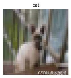

显示增强版图像样本

plt.figure(figsize=(10, 10))
for i in range(9):
    augmented_images = data_augmentation(np.array([image]))
    ax = plt.subplot(3, 3, i + 1)
    plt.imshow(augmented_images[0].numpy().astype("uint8"))
    plt.axis("off")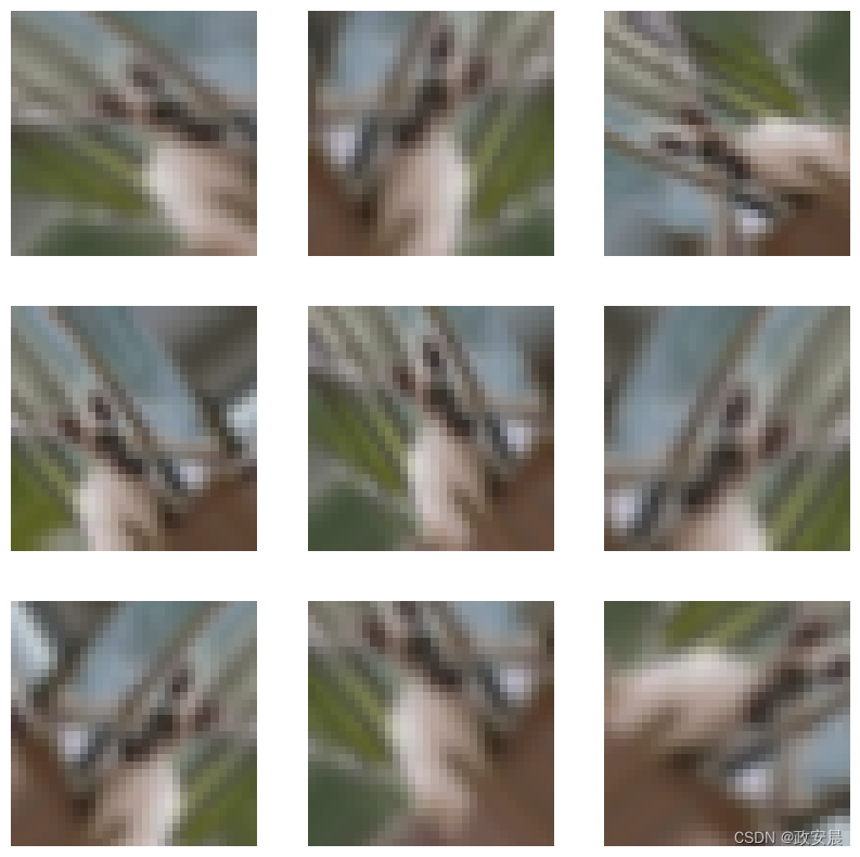

自我监督表征学习

实现视觉编码器

def create_encoder(representation_dim):
    encoder = keras.Sequential(
        [
            keras.applications.ResNet50V2(
                include_top=False, weights=None, pooling="avg"
            ),
            layers.Dense(representation_dim),
        ]
    )
    return encoder

实施无监督对比损失

class RepresentationLearner(keras.Model):
    def __init__(
        self,
        encoder,
        projection_units,
        num_augmentations,
        temperature=1.0,
        dropout_rate=0.1,
        l2_normalize=False,
        **kwargs
    ):
        super().__init__(**kwargs)
        self.encoder = encoder
        # Create projection head.
        self.projector = keras.Sequential(
            [
                layers.Dropout(dropout_rate),
                layers.Dense(units=projection_units, use_bias=False),
                layers.BatchNormalization(),
                layers.ReLU(),
            ]
        )
        self.num_augmentations = num_augmentations
        self.temperature = temperature
        self.l2_normalize = l2_normalize
        self.loss_tracker = keras.metrics.Mean(name="loss")

    @property
    def metrics(self):
        return [self.loss_tracker]

    def compute_contrastive_loss(self, feature_vectors, batch_size):
        num_augmentations = keras.ops.shape(feature_vectors)[0] // batch_size
        if self.l2_normalize:
            feature_vectors = keras.utils.normalize(feature_vectors)
        # The logits shape is [num_augmentations * batch_size, num_augmentations * batch_size].
        logits = (
            tf.linalg.matmul(feature_vectors, feature_vectors, transpose_b=True)
            / self.temperature
        )
        # Apply log-max trick for numerical stability.
        logits_max = keras.ops.max(logits, axis=1)
        logits = logits - logits_max
        # The shape of targets is [num_augmentations * batch_size, num_augmentations * batch_size].
        # targets is a matrix consits of num_augmentations submatrices of shape [batch_size * batch_size].
        # Each [batch_size * batch_size] submatrix is an identity matrix (diagonal entries are ones).
        targets = keras.ops.tile(
            tf.eye(batch_size), [num_augmentations, num_augmentations]
        )
        # Compute cross entropy loss
        return keras.losses.categorical_crossentropy(
            y_true=targets, y_pred=logits, from_logits=True
        )

    def call(self, inputs):
        # Preprocess the input images.
        preprocessed = data_preprocessing(inputs)
        # Create augmented versions of the images.
        augmented = []
        for _ in range(self.num_augmentations):
            augmented.append(data_augmentation(preprocessed))
        augmented = layers.Concatenate(axis=0)(augmented)
        # Generate embedding representations of the images.
        features = self.encoder(augmented)
        # Apply projection head.
        return self.projector(features)

    def train_step(self, inputs):
        batch_size = keras.ops.shape(inputs)[0]
        # Run the forward pass and compute the contrastive loss
        with tf.GradientTape() as tape:
            feature_vectors = self(inputs, training=True)
            loss = self.compute_contrastive_loss(feature_vectors, batch_size)
        # Compute gradients
        trainable_vars = self.trainable_variables
        gradients = tape.gradient(loss, trainable_vars)
        # Update weights
        self.optimizer.apply_gradients(zip(gradients, trainable_vars))
        # Update loss tracker metric
        self.loss_tracker.update_state(loss)
        # Return a dict mapping metric names to current value
        return {m.name: m.result() for m in self.metrics}

    def test_step(self, inputs):
        batch_size = keras.ops.shape(inputs)[0]
        feature_vectors = self(inputs, training=False)
        loss = self.compute_contrastive_loss(feature_vectors, batch_size)
        self.loss_tracker.update_state(loss)
        return {"loss": self.loss_tracker.result()}

训练模型

# Create vision encoder.
encoder = create_encoder(representation_dim)
# Create representation learner.
representation_learner = RepresentationLearner(
    encoder, projection_units, num_augmentations=2, temperature=0.1
)
# Create a a Cosine decay learning rate scheduler.
lr_scheduler = keras.optimizers.schedules.CosineDecay(
    initial_learning_rate=0.001, decay_steps=500, alpha=0.1
)
# Compile the model.
representation_learner.compile(
    optimizer=keras.optimizers.AdamW(learning_rate=lr_scheduler, weight_decay=0.0001),
    jit_compile=False,
)
# Fit the model.
history = representation_learner.fit(
    x=x_data,
    batch_size=512,
    epochs=50,  # for better results, increase the number of epochs to 500.
)

演绎展示：

Epoch 1/50
 118/118 ━━━━━━━━━━━━━━━━━━━━ 78s 187ms/step - loss: 557.1537
Epoch 2/50
 118/118 ━━━━━━━━━━━━━━━━━━━━ 19s 158ms/step - loss: 473.7576
Epoch 3/50
 118/118 ━━━━━━━━━━━━━━━━━━━━ 19s 160ms/step - loss: 204.2021
Epoch 4/50
 118/118 ━━━━━━━━━━━━━━━━━━━━ 19s 158ms/step - loss: 199.6705
Epoch 5/50
 118/118 ━━━━━━━━━━━━━━━━━━━━ 19s 158ms/step - loss: 199.4409
Epoch 6/50
 118/118 ━━━━━━━━━━━━━━━━━━━━ 19s 160ms/step - loss: 201.0644
Epoch 7/50
 118/118 ━━━━━━━━━━━━━━━━━━━━ 19s 159ms/step - loss: 199.7465
Epoch 8/50
 118/118 ━━━━━━━━━━━━━━━━━━━━ 19s 158ms/step - loss: 209.4148
Epoch 9/50
 118/118 ━━━━━━━━━━━━━━━━━━━━ 19s 160ms/step - loss: 200.9096
Epoch 10/50
 118/118 ━━━━━━━━━━━━━━━━━━━━ 19s 159ms/step - loss: 203.5660
Epoch 11/50
 118/118 ━━━━━━━━━━━━━━━━━━━━ 19s 158ms/step - loss: 197.5067
Epoch 12/50
 118/118 ━━━━━━━━━━━━━━━━━━━━ 19s 159ms/step - loss: 185.4315
Epoch 13/50
 118/118 ━━━━━━━━━━━━━━━━━━━━ 19s 159ms/step - loss: 196.7072
Epoch 14/50
 118/118 ━━━━━━━━━━━━━━━━━━━━ 19s 158ms/step - loss: 205.7930
Epoch 15/50
 118/118 ━━━━━━━━━━━━━━━━━━━━ 19s 158ms/step - loss: 196.2166
Epoch 16/50
 118/118 ━━━━━━━━━━━━━━━━━━━━ 19s 160ms/step - loss: 172.0755
Epoch 17/50
 118/118 ━━━━━━━━━━━━━━━━━━━━ 19s 158ms/step - loss: 153.7445
Epoch 18/50
 118/118 ━━━━━━━━━━━━━━━━━━━━ 19s 158ms/step - loss: 177.7372
Epoch 19/50
 118/118 ━━━━━━━━━━━━━━━━━━━━ 19s 161ms/step - loss: 149.0251
Epoch 20/50
 118/118 ━━━━━━━━━━━━━━━━━━━━ 19s 158ms/step - loss: 128.1759
Epoch 21/50
 118/118 ━━━━━━━━━━━━━━━━━━━━ 19s 157ms/step - loss: 122.5469
Epoch 22/50
 118/118 ━━━━━━━━━━━━━━━━━━━━ 19s 160ms/step - loss: 139.9140
Epoch 23/50
 118/118 ━━━━━━━━━━━━━━━━━━━━ 19s 158ms/step - loss: 135.2490
Epoch 24/50
 118/118 ━━━━━━━━━━━━━━━━━━━━ 19s 158ms/step - loss: 117.5860
Epoch 25/50
 118/118 ━━━━━━━━━━━━━━━━━━━━ 19s 160ms/step - loss: 117.3953
Epoch 26/50
 118/118 ━━━━━━━━━━━━━━━━━━━━ 19s 158ms/step - loss: 121.0800
Epoch 27/50
 118/118 ━━━━━━━━━━━━━━━━━━━━ 19s 158ms/step - loss: 108.4165
Epoch 28/50
 118/118 ━━━━━━━━━━━━━━━━━━━━ 19s 159ms/step - loss: 97.3604
Epoch 29/50
 118/118 ━━━━━━━━━━━━━━━━━━━━ 19s 159ms/step - loss: 88.7970
Epoch 30/50
 118/118 ━━━━━━━━━━━━━━━━━━━━ 19s 160ms/step - loss: 79.8381
Epoch 31/50
 118/118 ━━━━━━━━━━━━━━━━━━━━ 19s 157ms/step - loss: 69.1802
Epoch 32/50
 118/118 ━━━━━━━━━━━━━━━━━━━━ 21s 159ms/step - loss: 66.0070
Epoch 33/50
 118/118 ━━━━━━━━━━━━━━━━━━━━ 19s 158ms/step - loss: 62.4077
Epoch 34/50
 118/118 ━━━━━━━━━━━━━━━━━━━━ 19s 157ms/step - loss: 55.4975
Epoch 35/50
 118/118 ━━━━━━━━━━━━━━━━━━━━ 19s 160ms/step - loss: 51.2528
Epoch 36/50
 118/118 ━━━━━━━━━━━━━━━━━━━━ 19s 157ms/step - loss: 45.4217
Epoch 37/50
 118/118 ━━━━━━━━━━━━━━━━━━━━ 19s 157ms/step - loss: 39.3580
Epoch 38/50
 118/118 ━━━━━━━━━━━━━━━━━━━━ 19s 159ms/step - loss: 36.4156
Epoch 39/50
 118/118 ━━━━━━━━━━━━━━━━━━━━ 19s 157ms/step - loss: 33.9250
Epoch 40/50
 118/118 ━━━━━━━━━━━━━━━━━━━━ 19s 157ms/step - loss: 30.2516
Epoch 41/50
 118/118 ━━━━━━━━━━━━━━━━━━━━ 19s 159ms/step - loss: 25.0412
Epoch 42/50
 118/118 ━━━━━━━━━━━━━━━━━━━━ 19s 157ms/step - loss: 25.4968
Epoch 43/50
 118/118 ━━━━━━━━━━━━━━━━━━━━ 19s 157ms/step - loss: 22.3305
Epoch 44/50
 118/118 ━━━━━━━━━━━━━━━━━━━━ 19s 158ms/step - loss: 20.6767
Epoch 45/50
 118/118 ━━━━━━━━━━━━━━━━━━━━ 19s 157ms/step - loss: 20.2187
Epoch 46/50
 118/118 ━━━━━━━━━━━━━━━━━━━━ 18s 156ms/step - loss: 18.0097
Epoch 47/50
 118/118 ━━━━━━━━━━━━━━━━━━━━ 18s 156ms/step - loss: 17.4783
Epoch 48/50
 118/118 ━━━━━━━━━━━━━━━━━━━━ 19s 158ms/step - loss: 16.6550
Epoch 49/50
 118/118 ━━━━━━━━━━━━━━━━━━━━ 18s 156ms/step - loss: 16.0668
Epoch 50/50
 118/118 ━━━━━━━━━━━━━━━━━━━━ 18s 156ms/step - loss: 15.2431

绘图训练损失

plt.plot(history.history["loss"])
plt.ylabel("loss")
plt.xlabel("epoch")
plt.show()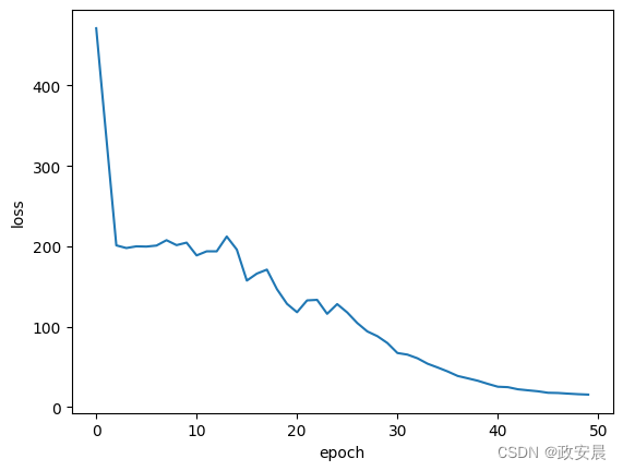

计算最近邻

生成图像的嵌入

batch_size = 500
# Get the feature vector representations of the images.
feature_vectors = encoder.predict(x_data, batch_size=batch_size, verbose=1)
# Normalize the feature vectores.
feature_vectors = keras.utils.normalize(feature_vectors)

演绎展示：

  19/120 ━━━[37m━━━━━━━━━━━━━━━━━  0s 9ms/step

WARNING: All log messages before absl::InitializeLog() is called are written to STDERR
I0000 00:00:1699918624.555770   94228 device_compiler.h:187] Compiled cluster using XLA!  This line is logged at most once for the lifetime of the process.

 120/120 ━━━━━━━━━━━━━━━━━━━━ 8s 9ms/step

为每个嵌入找到 k 个近邻

neighbours = []
num_batches = feature_vectors.shape[0] // batch_size
for batch_idx in tqdm(range(num_batches)):
    start_idx = batch_idx * batch_size
    end_idx = start_idx + batch_size
    current_batch = feature_vectors[start_idx:end_idx]
    # Compute the dot similarity.
    similarities = tf.linalg.matmul(current_batch, feature_vectors, transpose_b=True)
    # Get the indices of most similar vectors.
    _, indices = keras.ops.top_k(similarities, k=k_neighbours + 1, sorted=True)
    # Add the indices to the neighbours.
    neighbours.append(indices[..., 1:])

neighbours = np.reshape(np.array(neighbours), (-1, k_neighbours))

演绎展示：

100%|████████████████████████████████████████████████████████████████████████| 120/120 [00:17<00:00,  6.99it/s]

让我们在每一行显示一些邻居

nrows = 4
ncols = k_neighbours + 1

plt.figure(figsize=(12, 12))
position = 1
for _ in range(nrows):
    anchor_idx = np.random.choice(range(x_data.shape[0]))
    neighbour_indicies = neighbours[anchor_idx]
    indices = [anchor_idx] + neighbour_indicies.tolist()
    for j in range(ncols):
        plt.subplot(nrows, ncols, position)
        plt.imshow(x_data[indices[j]].astype("uint8"))
        plt.title(classes[y_data[indices[j]][0]])
        plt.axis("off")
        position += 1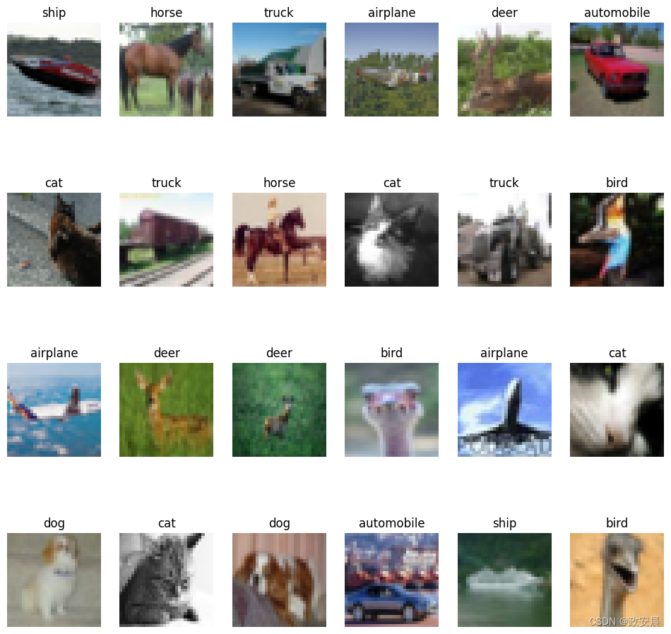

您注意到每一行的图像在视觉上都很相似，而且属于相似的类别。

利用近邻进行语义聚类

实施聚类一致性损失
该损耗试图确保邻域具有相同的聚类分配。

class ClustersConsistencyLoss(keras.losses.Loss):
    def __init__(self):
        super().__init__()

    def __call__(self, target, similarity, sample_weight=None):
        # Set targets to be ones.
        target = keras.ops.ones_like(similarity)
        # Compute cross entropy loss.
        loss = keras.losses.binary_crossentropy(
            y_true=target, y_pred=similarity, from_logits=True
        )
        return keras.ops.mean(loss)

实施聚类熵损失

该损失试图确保聚类分布大致均匀，以避免将大部分实例分配到一个聚类中。

class ClustersEntropyLoss(keras.losses.Loss):
    def __init__(self, entropy_loss_weight=1.0):
        super().__init__()
        self.entropy_loss_weight = entropy_loss_weight

    def __call__(self, target, cluster_probabilities, sample_weight=None):
        # Ideal entropy = log(num_clusters).
        num_clusters = keras.ops.cast(
            keras.ops.shape(cluster_probabilities)[-1], "float32"
        )
        target = keras.ops.log(num_clusters)
        # Compute the overall clusters distribution.
        cluster_probabilities = keras.ops.mean(cluster_probabilities, axis=0)
        # Replacing zero probabilities - if any - with a very small value.
        cluster_probabilities = keras.ops.clip(cluster_probabilities, 1e-8, 1.0)
        # Compute the entropy over the clusters.
        entropy = -keras.ops.sum(
            cluster_probabilities * keras.ops.log(cluster_probabilities)
        )
        # Compute the difference between the target and the actual.
        loss = target - entropy
        return loss

实施聚类模型

该模型将原始图像作为输入，使用训练有素的编码器生成其特征向量，并根据特征向量作为聚类分配生成聚类的概率分布。

def create_clustering_model(encoder, num_clusters, name=None):
    inputs = keras.Input(shape=input_shape)
    # Preprocess the input images.
    preprocessed = data_preprocessing(inputs)
    # Apply data augmentation to the images.
    augmented = data_augmentation(preprocessed)
    # Generate embedding representations of the images.
    features = encoder(augmented)
    # Assign the images to clusters.
    outputs = layers.Dense(units=num_clusters, activation="softmax")(features)
    # Create the model.
    model = keras.Model(inputs=inputs, outputs=outputs, name=name)
    return model

执行聚类学习器

该模型接收输入的锚图像及其邻近图像，使用聚类模型（clustering_model）为它们生成聚类分配，并产生两个输出结果：1. 相似度：锚图像与其邻近图像的聚类分配之间的相似度。该输出将被输入 ClustersConsistencyLoss。2. anchor_clustering：锚图像的聚类分配。该输出结果将反馈给聚类熵损失（ClustersEntropyLoss）。

def create_clustering_learner(clustering_model):
    anchor = keras.Input(shape=input_shape, name="anchors")
    neighbours = keras.Input(
        shape=tuple([k_neighbours]) + input_shape, name="neighbours"
    )
    # Changes neighbours shape to [batch_size * k_neighbours, width, height, channels]
    neighbours_reshaped = keras.ops.reshape(neighbours, tuple([-1]) + input_shape)
    # anchor_clustering shape: [batch_size, num_clusters]
    anchor_clustering = clustering_model(anchor)
    # neighbours_clustering shape: [batch_size * k_neighbours, num_clusters]
    neighbours_clustering = clustering_model(neighbours_reshaped)
    # Convert neighbours_clustering shape to [batch_size, k_neighbours, num_clusters]
    neighbours_clustering = keras.ops.reshape(
        neighbours_clustering,
        (-1, k_neighbours, keras.ops.shape(neighbours_clustering)[-1]),
    )
    # similarity shape: [batch_size, 1, k_neighbours]
    similarity = keras.ops.einsum(
        "bij,bkj->bik",
        keras.ops.expand_dims(anchor_clustering, axis=1),
        neighbours_clustering,
    )
    # similarity shape:  [batch_size, k_neighbours]
    similarity = layers.Lambda(
        lambda x: keras.ops.squeeze(x, axis=1), name="similarity"
    )(similarity)
    # Create the model.
    model = keras.Model(
        inputs=[anchor, neighbours],
        outputs=[similarity, anchor_clustering],
        name="clustering_learner",
    )
    return model

训练模型

# If tune_encoder_during_clustering is set to False,
# then freeze the encoder weights.
for layer in encoder.layers:
    layer.trainable = tune_encoder_during_clustering
# Create the clustering model and learner.
clustering_model = create_clustering_model(encoder, num_clusters, name="clustering")
clustering_learner = create_clustering_learner(clustering_model)
# Instantiate the model losses.
losses = [ClustersConsistencyLoss(), ClustersEntropyLoss(entropy_loss_weight=5)]
# Create the model inputs and labels.
inputs = {"anchors": x_data, "neighbours": tf.gather(x_data, neighbours)}
labels = np.ones(shape=(x_data.shape[0]))
# Compile the model.
clustering_learner.compile(
    optimizer=keras.optimizers.AdamW(learning_rate=0.0005, weight_decay=0.0001),
    loss=losses,
    jit_compile=False,
)

# Begin training the model.
clustering_learner.fit(x=inputs, y=labels, batch_size=512, epochs=50)

演绎展示：

Epoch 1/50
 118/118 ━━━━━━━━━━━━━━━━━━━━ 31s 109ms/step - loss: 0.3133
Epoch 2/50
 118/118 ━━━━━━━━━━━━━━━━━━━━ 10s 85ms/step - loss: 0.3133
Epoch 3/50
 118/118 ━━━━━━━━━━━━━━━━━━━━ 10s 84ms/step - loss: 0.3133
Epoch 4/50
 118/118 ━━━━━━━━━━━━━━━━━━━━ 10s 83ms/step - loss: 0.3133
Epoch 5/50
 118/118 ━━━━━━━━━━━━━━━━━━━━ 10s 83ms/step - loss: 0.3133
Epoch 6/50
 118/118 ━━━━━━━━━━━━━━━━━━━━ 10s 83ms/step - loss: 0.3133
Epoch 7/50
 118/118 ━━━━━━━━━━━━━━━━━━━━ 10s 83ms/step - loss: 0.3133
Epoch 8/50
 118/118 ━━━━━━━━━━━━━━━━━━━━ 10s 85ms/step - loss: 0.3133
Epoch 9/50
 118/118 ━━━━━━━━━━━━━━━━━━━━ 10s 84ms/step - loss: 0.3133
Epoch 10/50
 118/118 ━━━━━━━━━━━━━━━━━━━━ 10s 83ms/step - loss: 0.3133
Epoch 11/50
 118/118 ━━━━━━━━━━━━━━━━━━━━ 10s 83ms/step - loss: 0.3133
Epoch 12/50
 118/118 ━━━━━━━━━━━━━━━━━━━━ 10s 83ms/step - loss: 0.3133
Epoch 13/50
 118/118 ━━━━━━━━━━━━━━━━━━━━ 10s 83ms/step - loss: 0.3133
Epoch 14/50
 118/118 ━━━━━━━━━━━━━━━━━━━━ 10s 84ms/step - loss: 0.3133
Epoch 15/50
 118/118 ━━━━━━━━━━━━━━━━━━━━ 10s 83ms/step - loss: 0.3133
Epoch 16/50
 118/118 ━━━━━━━━━━━━━━━━━━━━ 10s 82ms/step - loss: 0.3133
Epoch 17/50
 118/118 ━━━━━━━━━━━━━━━━━━━━ 10s 83ms/step - loss: 0.3133
Epoch 18/50
 118/118 ━━━━━━━━━━━━━━━━━━━━ 10s 82ms/step - loss: 0.3133
Epoch 19/50
 118/118 ━━━━━━━━━━━━━━━━━━━━ 10s 81ms/step - loss: 0.3133
Epoch 20/50
 118/118 ━━━━━━━━━━━━━━━━━━━━ 10s 84ms/step - loss: 0.3133
Epoch 21/50
 118/118 ━━━━━━━━━━━━━━━━━━━━ 10s 83ms/step - loss: 0.3133
Epoch 22/50
 118/118 ━━━━━━━━━━━━━━━━━━━━ 10s 82ms/step - loss: 0.3133
Epoch 23/50
 118/118 ━━━━━━━━━━━━━━━━━━━━ 10s 81ms/step - loss: 0.3133
Epoch 24/50
 118/118 ━━━━━━━━━━━━━━━━━━━━ 10s 82ms/step - loss: 0.3133
Epoch 25/50
 118/118 ━━━━━━━━━━━━━━━━━━━━ 10s 82ms/step - loss: 0.3133
Epoch 26/50
 118/118 ━━━━━━━━━━━━━━━━━━━━ 10s 83ms/step - loss: 0.3133
Epoch 27/50
 118/118 ━━━━━━━━━━━━━━━━━━━━ 10s 83ms/step - loss: 0.3133
Epoch 28/50
 118/118 ━━━━━━━━━━━━━━━━━━━━ 10s 81ms/step - loss: 0.3133
Epoch 29/50
 118/118 ━━━━━━━━━━━━━━━━━━━━ 10s 81ms/step - loss: 0.3133
Epoch 30/50
 118/118 ━━━━━━━━━━━━━━━━━━━━ 10s 82ms/step - loss: 0.3133
Epoch 31/50
 118/118 ━━━━━━━━━━━━━━━━━━━━ 10s 82ms/step - loss: 0.3133
Epoch 32/50
 118/118 ━━━━━━━━━━━━━━━━━━━━ 10s 83ms/step - loss: 0.3133
Epoch 33/50
 118/118 ━━━━━━━━━━━━━━━━━━━━ 10s 83ms/step - loss: 0.3133
Epoch 34/50
 118/118 ━━━━━━━━━━━━━━━━━━━━ 10s 82ms/step - loss: 0.3133
Epoch 35/50
 118/118 ━━━━━━━━━━━━━━━━━━━━ 10s 81ms/step - loss: 0.3133
Epoch 36/50
 118/118 ━━━━━━━━━━━━━━━━━━━━ 10s 81ms/step - loss: 0.3133
Epoch 37/50
 118/118 ━━━━━━━━━━━━━━━━━━━━ 10s 82ms/step - loss: 0.3133
Epoch 38/50
 118/118 ━━━━━━━━━━━━━━━━━━━━ 10s 82ms/step - loss: 0.3133
Epoch 39/50
 118/118 ━━━━━━━━━━━━━━━━━━━━ 10s 84ms/step - loss: 0.3133
Epoch 40/50
 118/118 ━━━━━━━━━━━━━━━━━━━━ 10s 82ms/step - loss: 0.3133
Epoch 41/50
 118/118 ━━━━━━━━━━━━━━━━━━━━ 10s 81ms/step - loss: 0.3133
Epoch 42/50
 118/118 ━━━━━━━━━━━━━━━━━━━━ 10s 81ms/step - loss: 0.3133
Epoch 43/50
 118/118 ━━━━━━━━━━━━━━━━━━━━ 10s 82ms/step - loss: 0.3133
Epoch 44/50
 118/118 ━━━━━━━━━━━━━━━━━━━━ 10s 81ms/step - loss: 0.3133
Epoch 45/50
 118/118 ━━━━━━━━━━━━━━━━━━━━ 10s 84ms/step - loss: 0.3133
Epoch 46/50
 118/118 ━━━━━━━━━━━━━━━━━━━━ 10s 82ms/step - loss: 0.3133
Epoch 47/50
 118/118 ━━━━━━━━━━━━━━━━━━━━ 10s 81ms/step - loss: 0.3133
Epoch 48/50
 118/118 ━━━━━━━━━━━━━━━━━━━━ 10s 81ms/step - loss: 0.3133
Epoch 49/50
 118/118 ━━━━━━━━━━━━━━━━━━━━ 10s 82ms/step - loss: 0.3133
Epoch 50/50
 118/118 ━━━━━━━━━━━━━━━━━━━━ 10s 82ms/step - loss: 0.3133

<keras.src.callbacks.history.History at 0x7f629171c5b0>

绘图训练损失

plt.plot(history.history["loss"])
plt.ylabel("loss")
plt.xlabel("epoch")
plt.show()

聚类分析

将图像分配到群组

# Get the cluster probability distribution of the input images.
clustering_probs = clustering_model.predict(x_data, batch_size=batch_size, verbose=1)
# Get the cluster of the highest probability.
cluster_assignments = keras.ops.argmax(clustering_probs, axis=-1).numpy()
# Store the clustering confidence.
# Images with the highest clustering confidence are considered the 'prototypes'
# of the clusters.
cluster_confidence = keras.ops.max(clustering_probs, axis=-1).numpy()

演绎展示：

 120/120 ━━━━━━━━━━━━━━━━━━━━ 5s 13ms/step

让我们计算一下集群的大小

clusters = defaultdict(list)
for idx, c in enumerate(cluster_assignments):
    clusters[c].append((idx, cluster_confidence[idx]))

non_empty_clusters = defaultdict(list)
for c in clusters.keys():
    if clusters[c]:
        non_empty_clusters[c] = clusters[c]

for c in range(num_clusters):
    print("cluster", c, ":", len(clusters[c]))

演绎展示：
 

cluster 0 : 0
cluster 1 : 0
cluster 2 : 0
cluster 3 : 0
cluster 4 : 0
cluster 5 : 0
cluster 6 : 0
cluster 7 : 0
cluster 8 : 0
cluster 9 : 0
cluster 10 : 0
cluster 11 : 0
cluster 12 : 0
cluster 13 : 0
cluster 14 : 0
cluster 15 : 0
cluster 16 : 0
cluster 17 : 0
cluster 18 : 60000
cluster 19 : 0

聚类图像可视化

显示每个聚类的原型--聚类置信度最高的实例：

num_images = 8
plt.figure(figsize=(15, 15))
position = 1
for c in non_empty_clusters.keys():
    cluster_instances = sorted(
        non_empty_clusters[c], key=lambda kv: kv[1], reverse=True
    )

    for j in range(num_images):
        image_idx = cluster_instances[j][0]
        plt.subplot(len(non_empty_clusters), num_images, position)
        plt.imshow(x_data[image_idx].astype("uint8"))
        plt.title(classes[y_data[image_idx][0]])
        plt.axis("off")
        position += 1

计算聚类精度

首先，我们根据图像的多数标签为每个聚类分配一个标签。

然后，用具有多数标签的图像数量除以聚类的大小，计算出每个聚类的准确率。

cluster_label_counts = dict()

for c in range(num_clusters):
    cluster_label_counts[c] = [0] * num_classes
    instances = clusters[c]
    for i, _ in instances:
        cluster_label_counts[c][y_data[i][0]] += 1

    cluster_label_idx = np.argmax(cluster_label_counts[c])
    correct_count = np.max(cluster_label_counts[c])
    cluster_size = len(clusters[c])
    accuracy = (
        np.round((correct_count / cluster_size) * 100, 2) if cluster_size > 0 else 0
    )
    cluster_label = classes[cluster_label_idx]
    print("cluster", c, "label is:", cluster_label, " -  accuracy:", accuracy, "%")

cluster 0 label is: airplane  -  accuracy: 0 %
cluster 1 label is: airplane  -  accuracy: 0 %
cluster 2 label is: airplane  -  accuracy: 0 %
cluster 3 label is: airplane  -  accuracy: 0 %
cluster 4 label is: airplane  -  accuracy: 0 %
cluster 5 label is: airplane  -  accuracy: 0 %
cluster 6 label is: airplane  -  accuracy: 0 %
cluster 7 label is: airplane  -  accuracy: 0 %
cluster 8 label is: airplane  -  accuracy: 0 %
cluster 9 label is: airplane  -  accuracy: 0 %
cluster 10 label is: airplane  -  accuracy: 0 %
cluster 11 label is: airplane  -  accuracy: 0 %
cluster 12 label is: airplane  -  accuracy: 0 %
cluster 13 label is: airplane  -  accuracy: 0 %
cluster 14 label is: airplane  -  accuracy: 0 %
cluster 15 label is: airplane  -  accuracy: 0 %
cluster 16 label is: airplane  -  accuracy: 0 %
cluster 17 label is: airplane  -  accuracy: 0 %
cluster 18 label is: airplane  -  accuracy: 10.0 %
cluster 19 label is: airplane  -  accuracy: 0 %

结论

为了提高准确度，您可以：

1) 增加表征学习和聚类阶段的历时次数；

2) 允许在聚类阶段调整编码器权重；

3) 如 SCAN 原始论文所述，通过自标记执行最后的微调步骤。

请注意，我们并不期望无监督图像聚类技术能够超越有监督图像分类技术的准确性，而是希望它们能够学习图像的语义，并将其归入与原始类别相似的聚类中。

---