一、数据集为firm.csv,给出了22家美国公用事业公司的相关数据集,各数据集变量的名称和含义如下:X1为固定费用周转比(收入/债务),X2为资本回报率,X3为每千瓦容量成本,X4为年载荷因子,X5为1974-1975年高峰期千瓦时增长需求,X6为销售量(年千瓦时用量),X7为核能所占百分比。
| X1 | X2 | X3 | X4 | X5 | X6 | X7 |
| 1.06 | 9.2 | 151 | 54.4 | 1.6 | 9077 | 0 |
| 0.89 | 10.3 | 202 | 57.9 | 2.2 | 5088 | 25.3 |
| 1.43 | 15.4 | 113 | 53 | 3.4 | 9212 | 0 |
| 1.02 | 11.2 | 168 | 56 | 0.3 | 6423 | 34.3 |
| 1.49 | 8.8 | 192 | 51.2 | 1 | 3300 | 15.6 |
| 1.32 | 13.5 | 111 | 60 | -2.2 | 11127 | 22.5 |
| 1.22 | 12.2 | 175 | 67.6 | 2.2 | 7642 | 0 |
| 1.1 | 9.2 | 245 | 57 | 3.3 | 13082 | 0 |
| 1.34 | 13 | 168 | 60.4 | 7.2 | 8406 | 0 |
| 1.12 | 12.4 | 197 | 53 | 2.7 | 6455 | 39.2 |
| 0.75 | 7.5 | 173 | 51.5 | 6.5 | 17441 | 0 |
| 1.13 | 10.9 | 178 | 62 | 3.7 | 6154 | 0 |
| 1.15 | 12.7 | 199 | 53.7 | 6.4 | 7179 | 50.2 |
| 1.09 | 12 | 96 | 49.8 | 1.4 | 9673 | 0 |
| 0.96 | 7.6 | 164 | 62.2 | -0.1 | 6468 | 0.9 |
| 1.16 | 9.9 | 252 | 56 | 9.2 | 15991 | 0 |
| 0.76 | 6.4 | 136 | 61.9 | 9 | 5714 | 8.3 |
| 1.05 | 12.6 | 150 | 56.7 | 2.7 | 10140 | 0 |
| 1.16 | 11.7 | 104 | 54 | -2.1 | 13507 | 0 |
| 1.2 | 11.8 | 148 | 59.9 | 3.5 | 7287 | 41.1 |
| 1.04 | 8.6 | 204 | 61 | 3.5 | 6650 | 0 |
| 1.07 | 9.3 | 174 | 54.3 | 5.9 | 10093 | 26.6 |
二、导入分析包和数据集,指定数据集的变量类型
library(ggplot2)
library(ggpubr)
install.packages('ggpubr')
library(ggpubr)
firm<-read.csv('f:\\桌面\\firm.csv',colClasses = c(rep('numeric',7)))
firm
三、对数据进行标准化
stdfirm<-scale(firm,center=T,scale=T)
stdfirm
运行得到:
stdfirm<-scale(firm,center=T,scale=T)
> stdfirm
               X1          X2           X3          X4          X5          X6         X7
 [1,] -0.29315791 -0.68463896 -0.417122002 -0.57771516 -0.52622751  0.04590290 -0.7146294
 [2,] -1.21451134 -0.19445367  0.821002037  0.20683629 -0.33381191 -1.07776413  0.7920476
 [3,]  1.71214073  2.07822360 -1.339645796 -0.89153574  0.05101929  0.08393124 -0.7146294
 [4,] -0.50994695  0.20660702 -0.004413989 -0.21906307 -0.94312798 -0.70170610  1.3280197
 [5,]  2.03732429 -0.86288816  0.578232617 -1.29501935 -0.71864311 -1.58142837  0.2143888
 [6,]  1.11597086  1.23153991 -1.388199680  0.67756716 -1.74485965  0.62337028  0.6253007
 [7,]  0.57399826  0.65223002  0.165524604  2.38116460 -0.33381191 -0.35832428 -0.7146294
 [8,] -0.07636887 -0.68463896  1.864910540  0.00509449  0.01895002  1.17407698 -0.7146294
 [9,]  1.22436538  1.00872841 -0.004413989  0.76723019  1.26965142 -0.14311204 -0.7146294
[10,]  0.03202565  0.74135462  0.699617327 -0.89153574 -0.17346558 -0.69269198  1.6198267
[11,] -1.97327298 -1.44219805  0.116970720 -1.22777208  1.04516655  2.40196983 -0.7146294
[12,]  0.08622291  0.07292013  0.238355430  1.12588228  0.14722709 -0.77748109 -0.7146294
[13,]  0.19461744  0.87504152  0.748171211 -0.73462545  1.01309729 -0.48874740  2.2749037
[14,] -0.13056613  0.56310542 -1.752353809 -1.60883993 -0.59036605  0.21379097 -0.7146294
[15,] -0.83513051 -1.39763576 -0.101521757  1.17071379 -1.07140505 -0.68902999 -0.6610322
[16,]  0.24881470 -0.37270287  2.034849134 -0.21906307  1.91103676  1.99351729 -0.7146294
[17,] -1.91907572 -1.93238335 -0.781276132  1.10346652  1.84689822 -0.90142531 -0.2203441
[18,] -0.34735517  0.83047922 -0.441398944 -0.06215278 -0.17346558  0.34534086 -0.7146294
[19,]  0.24881470  0.42941852 -1.558138274 -0.66737818 -1.71279038  1.29379583 -0.7146294
[20,]  0.46560374  0.47398082 -0.489952828  0.65515141  0.08308855 -0.45832473  1.7329764
[21,] -0.40155243 -0.95201276  0.869555920  0.90172472  0.08308855 -0.63776215 -0.7146294
[22,] -0.23896065 -0.64007666  0.141247662 -0.60013092  0.85275095  0.33210137  0.8694658
attr(,"scaled:center")
         X1          X2          X3          X4          X5          X6          X7
   1.114091   10.736364  168.181818   56.977273    3.240909 8914.045455   12.000000
attr(,"scaled:scale")
          X1           X2           X3           X4           X5           X6           X7
   0.1845112    2.2440494   41.1913495    4.4611478    3.1182503 3549.9840305   16.7919198
四、进行K均值聚类分析
指定类别K=3,最低迭代次数为99次,进行25次随机初始化。
stdfirm.kmeans<-kmeans(stdfirm,centers=3,iter.max=99,nstart = 25)
查看聚类的结果:
names(stdfirm.kmeans)
1、stdfirm.kmeans$cluster
得到聚类结果:
stdfirm.kmeans$cluster
 [1] 3 3 2 3 3 2 3 1 3 3 1 3 3 2 3 1 3 2 2 3 3 3
2、stdfirm.kmeans$centers
得到聚类后的3个中心
stdfirm.kmeans$centers
          X1         X2        X3         X4          X5         X6         X7
1 -0.6002757 -0.8331800  1.338910 -0.4805802  0.99171778  1.8565214 -0.7146294
2  0.5198010  1.0265533 -1.295947 -0.5104679 -0.83409247  0.5120458 -0.4466434
3 -0.0570127 -0.1880876  0.175929  0.2852914  0.08537922 -0.5806995  0.3126504
3、stdfirm.kmeans$totss
得到总平方和
stdfirm.kmeans$totss
[1] 147
4、stdfirm.kmeans$tot.withinss
得到组内平方和
 stdfirm.kmeans$tot.withinss
[1] 92.53055
5、stdfirm.kmeans$betweenss
得到组间平方和
6、stdfirm.kmeans$size
得到各类别的观测数
stdfirm.kmeans$size
[1]  3  5 14
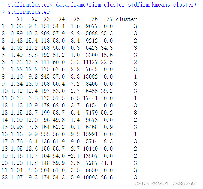
7、将聚类结果保存在原始数据集firm.csv中
stdfirm.kmeans.cluster<-stdfirm.kmeans$cluster
stdfirmcluster<-data.frame(firm,cluster=stdfirm.kmeans.cluster)
stdfirmcluster
运行得到:
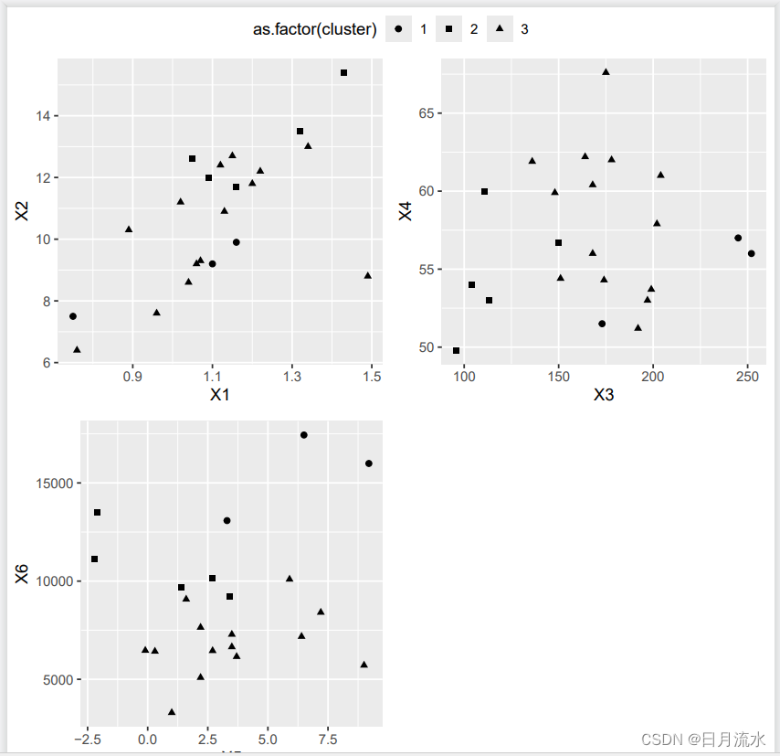
7、聚类结果可视化
绘制出变量X1和X2,X3和X4,X5和X6样本散点图,并保存在文档中。
本次聚类分析中指定了聚类中心为K=3
pdf('f:/桌面/stdfirm.kmeans.pdf')
p1<-ggplot(stdfirmcluster,aes(x=X1,y=X2,shape=as.factor(cluster)))+
geom_point()+scale_shape_manual(values = c('circle','square','triangle'))
p2<-ggplot(stdfirmcluster,aes(x=X3,y=X4,shape=as.factor(cluster)))+
geom_point()+scale_shape_manual(values = c('circle','square','triangle'))
p3<-ggplot(stdfirmcluster,aes(x=X5,y=X6,shape=as.factor(cluster)))+
geom_point()+scale_shape_manual(values = c('circle','square','triangle'))
ggarrange(p1,p2,p3,ncol=2,nrow = 2,common.legend=T)
dev.off()
运行得到:
五、进行系统聚类分析
1、使用系统聚类函数hclust()进行聚类分析,默认使用各样本的距离矩阵,指定使用平均距离法
firm_hclust<-hclust(dist(stdfirm),method='average')
2、绘制聚类树形图:
plot(firm_hclust)
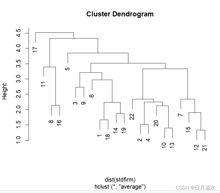
3、指定聚类数为3,并在聚类树中标注出来
firm.hlust.cluster<-cutree(firm_hclust,k=3)
rect.hclust(firm_hclust,k=3)
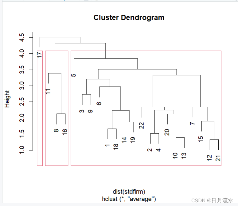
4、得到聚类结果
 firm.hlust.cluster<-cutree(firm_hclust,k=3)
> firm.hlust.cluster
 [1] 1 1 1 1 1 1 1 2 1 1 2 1 1 1 1 2 3 1 1 1 1 1
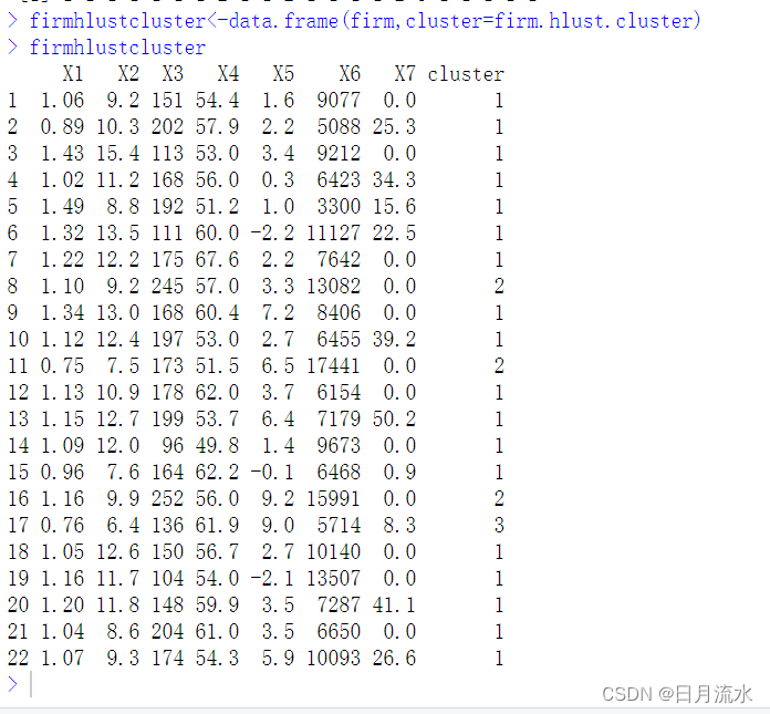
5、将聚类结果加到原始数据集中
firmhlustcluster<-data.frame(firm,cluster=firm.hlust.cluster)
firmhlustcluster
6、聚类结果可视化
绘制出变量X1和X2,X3和X4,X5和X6样本散点图,并保存在文档中。
pdf('f:/桌面/firm_cluster.pdf')
p4<-ggplot(firmhlustcluster,aes(x=X1,y=X2,shape=as.factor(cluster)))+
geom_point()+scale_shape_manual(values=c('circle','square','triangle'))
p5<-ggplot(firmhlustcluster,aes(x=X3,y=X4,shape=as.factor(cluster)))+
geom_point()+scale_shape_manual(values=c('circle','square','triangle'))
p6<-ggplot(firmhlustcluster,aes(x=X5,y=X6,shape=as.factor(cluster)))+
geom_point()+scale_shape_manual(values=c('circle','square','triangle'))
ggarrange(p4,p5,p6,ncol=2,nrow = 2,common.legend=T)
dev.off()
 六、使用R软件程序包NbClust进行聚类分析,程序包中的NbClust()函数提供最佳类别数的30种统计方法,综合各种最佳类别数的统计指标来给出最佳类别数的判断,下面是初步的介绍。
这里的聚类方法可以是Kmeans,也可以是系统聚类法中的average。
install.packages('NbClust')
library(NbClust)
1、NbClust()函数进行K均值聚类分析
firm.nbclust.kmeans<-NbClust(stdfirm,method='kmeans')
运行得到:
firm.nbclust.kmeans<-NbClust(stdfirm,method='kmeans')
*** : The Hubert index is a graphical method of determining the number of clusters.
                In the plot of Hubert index, we seek a significant knee that corresponds to a
                significant increase of the value of the measure i.e the significant peak in Hubert
                index second differences plot.

*** : The D index is a graphical method of determining the number of clusters.
                In the plot of D index, we seek a significant knee (the significant peak in Dindex
                second differences plot) that corresponds to a significant increase of the value of
                the measure.

*******************************************************************
* Among all indices:
* 4 proposed 2 as the best number of clusters
* 4 proposed 3 as the best number of clusters
* 6 proposed 4 as the best number of clusters
* 1 proposed 5 as the best number of clusters
* 1 proposed 6 as the best number of clusters
* 1 proposed 8 as the best number of clusters
* 1 proposed 13 as the best number of clusters
* 5 proposed 15 as the best number of clusters

                   ***** Conclusion *****

* According to the majority rule, the best number of clusters is  4


*******************************************************************
Warning messages:
1: In pf(beale, pp, df2) : 产生了NaNs
2: In pf(beale, pp, df2) : 产生了NaNs
3: In pf(beale, pp, df2) : 产生了NaNs
上面的说明According to the majority rule, the best number of clusters is 4,大多数的类别判别指标给出的类别结果为4个类别。
需要说明的是Hubert index和 D index可以使用图形来进行类别判别,运行得到的图像为:
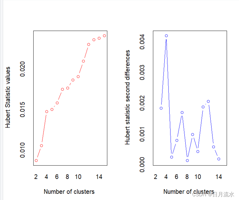

第二张图即为这两个指标的二阶差分图,从判别指标的二阶差分图中的峰值即可判别最佳类别数为4个类别。
2、查看firm.nbclust.kmeans均值聚类分析的结果
names(firm.nbclust.kmeans)
运行得到:
names(firm.nbclust.kmeans)
[1] "All.index"          "All.CriticalValues" "Best.nc"            "Best.partition"
firm.nbclust.kmeans$All.index
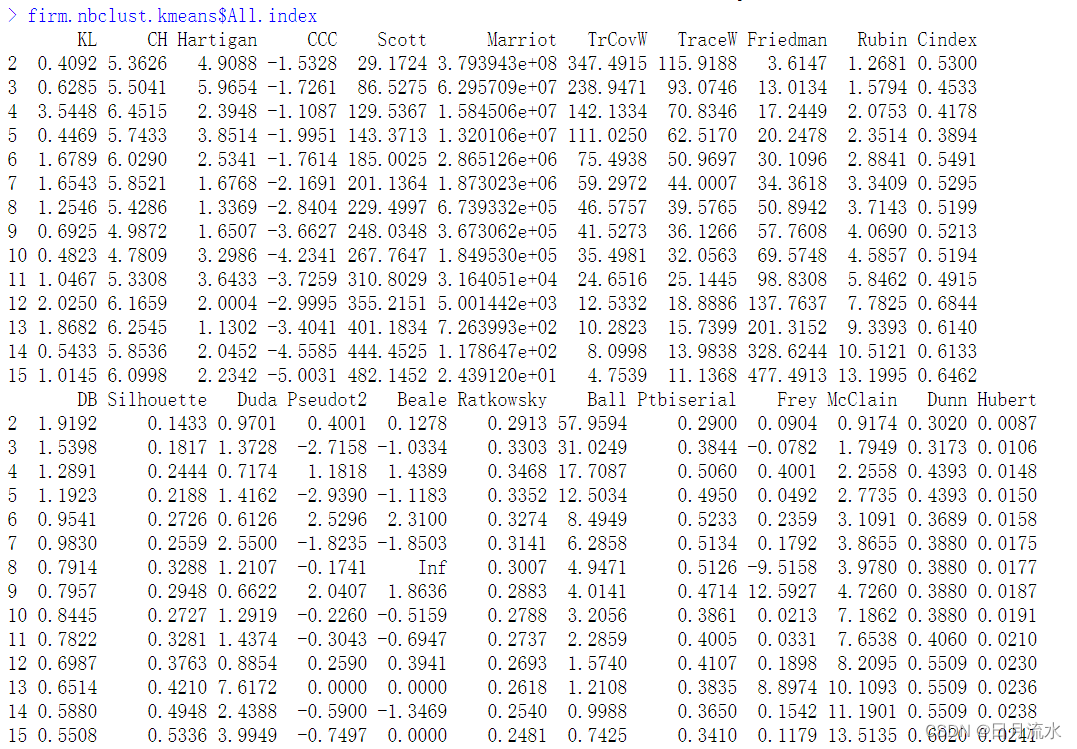
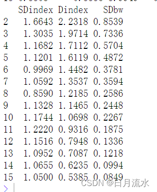
该命令给出了各类别判别指标在各类别下的指标值。
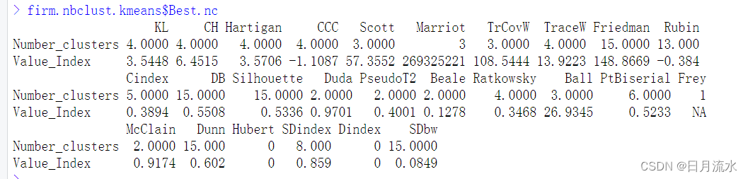
firm.nbclust.kmeans$Best.nc
该命令给出了各判别指标给出了具体的最佳类别判别数和在该类别下的判别指标值
irm.nbclust.kmeans$Best.partition
给出来最佳判别数下的给样本所属的类别
firm.nbclust.kmeans$Best.partition
 [1] 2 1 2 1 1 2 4 3 4 1 3 4 1 2 4 3 4 2 2 1 4 1
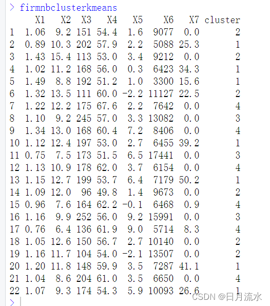
3、把聚类结果加入到原始数据中
firm.nbclust.kmeans.cluster<-firm.nbclust.kmeans$Best.partition
firmnbclusterkmeans<-data.frame(firm,cluster=firm.nbclust.kmeans.cluster)
firmnbclusterkmeans
4、使用NbClust()函数进行系统聚类分析
firm.nbclust.average<-NbClust(stdfirm,method='average')
According to the majority rule, the best number of clusters is 3
此次进行聚类分析,得到最佳的类别为3个类别。
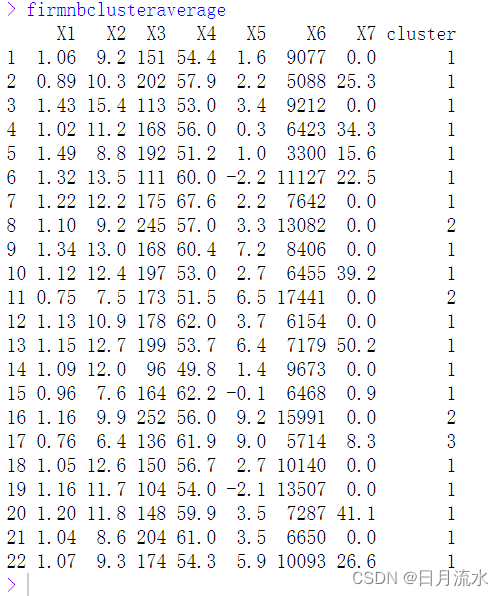
把距离结果加入在原始数据中
firm.nbclust.average.cluster<-firm.nbclust.average$Best.partition
firmnbclusteraverage<-data.frame(firm,cluster=firm.nbclust.average.cluster)
firmnbclusteraverage