参考:
https://zh-v2.d2l.ai/chapter_computer-vision/multiscale-object-detection.html
R-CNN 及系列
区域卷积神经网络 region-based CNN
R-CNN
R-CNN首先从输入图像中选取若干(例如2000个)提议区域,并标注它们的类别和边界框(如偏移量)。用卷积神经网络对每个提议区域进行前向传播以抽取其特征。 接下来,我们用每个提议区域的特征来预测类别和边界框。
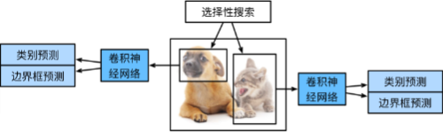
R-CNN步骤:
对每张图选择多个区域,然后每个区域作为一个样本,进入CNN抽取特征,最后多个SVM分类器分类,判断是否属于某个类别。回归模型得到更准确的边框
尽管R-CNN模型通过预训练的卷积神经网络有效地抽取了图像特征,但它的速度很慢。
Fast R-CNN
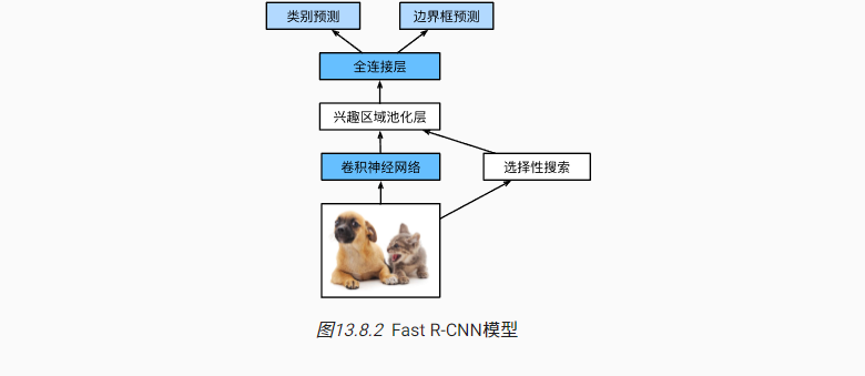
改进:R-CNN有大量区域可能是相互覆盖的,每次重新抽取特征过于浪费。因此Fast R-CNN先对输入图片抽取特征,再选区域
代替R-CNN使用多个SVM做分类,而是使用单个多累逻辑回归
Faster R-CNN
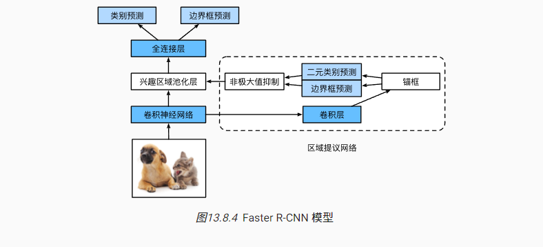
将selective search替换为region proposal network,
1.使用填充为1的3*3的卷积层变换卷积神经网络的输出,并将输出通道数记为c。这样,卷积神经网络为图像抽取的特征图中的每个单元均得到一个长度为c的新特征.
2.以特征图的每个像素为中心,生成多个不同大小和宽高比的锚框并标注它们.
3.使用锚框中心单元长度为C的特征,分别预测该锚框的二元类别(含目标还是背景)和边界框.
4.使用非极大值抑制,从预测类别为目标的预测边界框中移除相似的结果。最终输出的预测边界框即是兴趣区域汇聚层所需的提议区域.
用于对象实例分割,,该框架通过添加一个用于预测物体掩码的分支与用于边界框识别的现有分支并行添加了用于预测物体掩码的分支来扩展Faster R-CNN
Faster R-CNN :检测模型,使用 region proposal network (RPN)生成边界框。RPN 经过训练,可以预测物体出现在图像中每个位置的可能性,并生成一组候选方框。然后使用单独的网络对这些候选框进行优化,该网络可以预测精确的物体边界。
作为端到端训练的结果,区域提议网络能够学习到如何生成高质量的提议区域,从而在减少了从数据中学习的提议区域的数量的情况下,仍保持目标检测的精度。它不适用于像素-像素分类。
Mask R-CNN
在Faster R-CNN上加入了一个新的像素级别的预测层,不仅对一个锚框预测它对应的类和真实边框,还会判断锚框内每个像素对应的是哪个物体还是背景
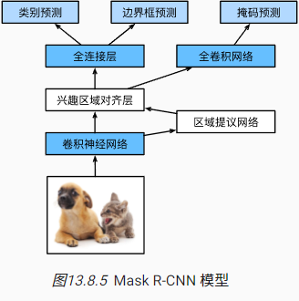
Mask R-CNN是基于Faster R-CNN修改而来的。 具体来说,Mask R-CNN将兴趣区域汇聚层替换为了 兴趣区域对齐层,使用双线性插值(bilinear interpolation)来保留特征图上的空间信息,从而更适于像素级预测。
兴趣区域对齐层的输出包含了所有与兴趣区域的形状相同的特征图。 它们不仅被用于预测每个兴趣区域的类别和边界框,还通过额外的全卷积网络预测目标的像素级位置。
目标检测和边界框
目标检测:
在图像分类任务中,我们假设图像中只有一个主要物体对象,我们只关注如何识别其类别。
然而,很多时候图像里有多个我们感兴趣的目标,我们不仅想知道它们的类别,还想得到它们在图像中的具体位置。
边界框
使用边界框bounding box描述对象的空间位置。边界框是矩形的,由矩形左上角的以及右下角x和y坐标决定。
可以在两种常用的边界框表示(中间,宽度,高度)和(左上,右下)坐标之间进行转换。
#@save
def box_corner_to_center(boxes):
    """从(左上,右下)转换到(中间,宽度,高度)"""
    x1, y1, x2, y2 = boxes[:, 0], boxes[:, 1], boxes[:, 2], boxes[:, 3]
    cx = (x1 + x2) / 2
    cy = (y1 + y2) / 2
    w = x2 - x1
    h = y2 - y1
    boxes = torch.stack((cx, cy, w, h), axis=-1)
    return boxes

#@save
def box_center_to_corner(boxes):
    """从(中间,宽度,高度)转换到(左上,右下)"""
    cx, cy, w, h = boxes[:, 0], boxes[:, 1], boxes[:, 2], boxes[:, 3]
    x1 = cx - 0.5 * w
    y1 = cy - 0.5 * h
    x2 = cx + 0.5 * w
    y2 = cy + 0.5 * h
    boxes = torch.stack((x1, y1, x2, y2), axis=-1)
    return boxes

#@save
def bbox_to_rect(bbox, color):
    # 将边界框(左上x,左上y,右下x,右下y)格式转换成matplotlib格式:
    # ((左上x,左上y),宽,高)
    return d2l.plt.Rectangle(
        xy=(bbox[0], bbox[1]), width=bbox[2]-bbox[0], height=bbox[3]-bbox[1],
        fill=False, edgecolor=color, linewidth=2)
# bbox是边界框的英文缩写
dog_bbox, cat_bbox = [60.0, 45.0, 378.0, 516.0], [400.0, 112.0, 655.0, 493.0]
图像中坐标的原点是图像的左上角,向右的方向为x轴的正方向,向下的方向为y轴的正方向。
锚框
目标检测算法通常会在输入图像中采样大量的区域,然后判断这些区域中是否包含我们感兴趣的目标,并调整区域边界从而更准确地预测目标的真实边界框(ground-truth bounding box)。
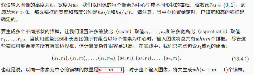
不同的模型使用的区域采样方法可能不同。 这里我们介绍其中的一种方法:以每个像素为中心,生成多个缩放比和宽高比(aspect ratio)不同的边界框。
生成多个锚框
#@save
def multibox_prior(data, sizes, ratios):
    """生成以每个像素为中心具有不同形状的锚框"""
    in_height, in_width = data.shape[-2:]
    device, num_sizes, num_ratios = data.device, len(sizes), len(ratios)
    boxes_per_pixel = (num_sizes + num_ratios - 1)
    size_tensor = torch.tensor(sizes, device=device)
    ratio_tensor = torch.tensor(ratios, device=device)

    # 为了将锚点移动到像素的中心,需要设置偏移量。
    # 因为一个像素的高为1且宽为1,我们选择偏移我们的中心0.5
    offset_h, offset_w = 0.5, 0.5
    steps_h = 1.0 / in_height  # 在y轴上缩放步长
    steps_w = 1.0 / in_width  # 在x轴上缩放步长

    # 生成锚框的所有中心点
    center_h = (torch.arange(in_height, device=device) + offset_h) * steps_h
    center_w = (torch.arange(in_width, device=device) + offset_w) * steps_w
    shift_y, shift_x = torch.meshgrid(center_h, center_w, indexing='ij')
    shift_y, shift_x = shift_y.reshape(-1), shift_x.reshape(-1)

    # 生成“boxes_per_pixel”个高和宽,
    # 之后用于创建锚框的四角坐标(xmin,xmax,ymin,ymax)
    w = torch.cat((size_tensor * torch.sqrt(ratio_tensor[0]),
                   sizes[0] * torch.sqrt(ratio_tensor[1:])))\
                   * in_height / in_width  # 处理矩形输入
    h = torch.cat((size_tensor / torch.sqrt(ratio_tensor[0]),
                   sizes[0] / torch.sqrt(ratio_tensor[1:])))
    # 除以2来获得半高和半宽
    anchor_manipulations = torch.stack((-w, -h, w, h)).T.repeat(
                                        in_height * in_width, 1) / 2

    # 每个中心点都将有“boxes_per_pixel”个锚框,
    # 所以生成含所有锚框中心的网格,重复了“boxes_per_pixel”次
    out_grid = torch.stack([shift_x, shift_y, shift_x, shift_y],
                dim=1).repeat_interleave(boxes_per_pixel, dim=0)
    output = out_grid + anchor_manipulations
    return output.unsqueeze(0)
锚框变量Y的形状是(批量大小,锚框的数量,4)
交并比(intersection over union,IoU)
衡量锚框和真实边界框之间的相似性。 杰卡德系数(Jaccard)可以衡量两组之间的相似性。杰卡德系数是他们交集的大小除以他们并集的大小:

交并比的取值范围在0和1之间:0表示两个边界框无重合像素,1表示两个边界框完全重合。
box_iou函数将在这两个列表中计算它们成对的交并比
#@save
def box_iou(boxes1, boxes2):
    """计算两个锚框或边界框列表中成对的交并比"""
    box_area = lambda boxes: ((boxes[:, 2] - boxes[:, 0]) *
                              (boxes[:, 3] - boxes[:, 1]))
    # boxes1,boxes2,areas1,areas2的形状:
    # boxes1:(boxes1的数量,4),
    # boxes2:(boxes2的数量,4),
    # areas1:(boxes1的数量,),
    # areas2:(boxes2的数量,)
    areas1 = box_area(boxes1)
    areas2 = box_area(boxes2)
    # inter_upperlefts,inter_lowerrights,inters的形状:
    # (boxes1的数量,boxes2的数量,2)
    inter_upperlefts = torch.max(boxes1[:, None, :2], boxes2[:, :2])
    inter_lowerrights = torch.min(boxes1[:, None, 2:], boxes2[:, 2:])
    inters = (inter_lowerrights - inter_upperlefts).clamp(min=0)
    # inter_areasandunion_areas的形状:(boxes1的数量,boxes2的数量)
    inter_areas = inters[:, :, 0] * inters[:, :, 1]
    union_areas = areas1[:, None] + areas2 - inter_areas
    return inter_areas / union_areas
在训练数据中标注锚框
为了训练目标检测模型,我们需要每个锚框的类别(class)和偏移量(offset)标签,其中前者是与锚框相关的对象的类别,后者是真实边界框相对于锚框的偏移量。 在预测时,我们为每个图像生成多个锚框,预测所有锚框的类别和偏移量,根据预测的偏移量调整它们的位置以获得预测的边界框,最后只输出符合特定条件的预测边界框。
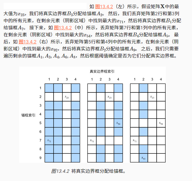
- 将真实边界框分配给锚框
#@save
def assign_anchor_to_bbox(ground_truth, anchors, device, iou_threshold=0.5):
    """将最接近的真实边界框分配给锚框"""
    num_anchors, num_gt_boxes = anchors.shape[0], ground_truth.shape[0]
    # 位于第i行和第j列的元素x_ij是锚框i和真实边界框j的IoU
    jaccard = box_iou(anchors, ground_truth)
    # 对于每个锚框,分配的真实边界框的张量
    anchors_bbox_map = torch.full((num_anchors,), -1, dtype=torch.long,
                                  device=device)
    # 根据阈值,决定是否分配真实边界框
    max_ious, indices = torch.max(jaccard, dim=1)
    anc_i = torch.nonzero(max_ious >= iou_threshold).reshape(-1)
    box_j = indices[max_ious >= iou_threshold]
    anchors_bbox_map[anc_i] = box_j
    col_discard = torch.full((num_anchors,), -1)
    row_discard = torch.full((num_gt_boxes,), -1)
    for _ in range(num_gt_boxes):
        max_idx = torch.argmax(jaccard)
        box_idx = (max_idx % num_gt_boxes).long()
        anc_idx = (max_idx / num_gt_boxes).long()
        anchors_bbox_map[anc_idx] = box_idx
        jaccard[:, box_idx] = col_discard
        jaccard[anc_idx, :] = row_discard
    return anchors_bbox_map
- 标记类别和偏移量
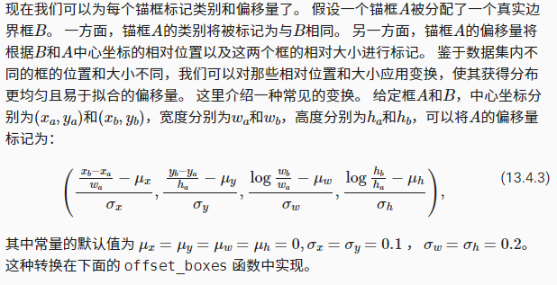
如果一个锚框没有被分配真实边界框,我们只需将锚框的类别标记为背景
#@save
def offset_boxes(anchors, assigned_bb, eps=1e-6):
    """对锚框偏移量的转换"""
    c_anc = d2l.box_corner_to_center(anchors)
    c_assigned_bb = d2l.box_corner_to_center(assigned_bb)
    offset_xy = 10 * (c_assigned_bb[:, :2] - c_anc[:, :2]) / c_anc[:, 2:]
    offset_wh = 5 * torch.log(eps + c_assigned_bb[:, 2:] / c_anc[:, 2:])
    offset = torch.cat([offset_xy, offset_wh], axis=1)
    return offset

#@save
def multibox_target(anchors, labels):
    """使用真实边界框标记锚框"""
    batch_size, anchors = labels.shape[0], anchors.squeeze(0)
    batch_offset, batch_mask, batch_class_labels = [], [], []
    device, num_anchors = anchors.device, anchors.shape[0]
    for i in range(batch_size):
        label = labels[i, :, :]
        anchors_bbox_map = assign_anchor_to_bbox(
            label[:, 1:], anchors, device)
        bbox_mask = ((anchors_bbox_map >= 0).float().unsqueeze(-1)).repeat(
            1, 4)
        # 将类标签和分配的边界框坐标初始化为零
        class_labels = torch.zeros(num_anchors, dtype=torch.long,
                                   device=device)
        assigned_bb = torch.zeros((num_anchors, 4), dtype=torch.float32,
                                  device=device)
        # 使用真实边界框来标记锚框的类别。
        # 如果一个锚框没有被分配,标记其为背景(值为零)
        indices_true = torch.nonzero(anchors_bbox_map >= 0)
        bb_idx = anchors_bbox_map[indices_true]
        class_labels[indices_true] = label[bb_idx, 0].long() + 1
        assigned_bb[indices_true] = label[bb_idx, 1:]
        # 偏移量转换
        offset = offset_boxes(anchors, assigned_bb) * bbox_mask
        batch_offset.append(offset.reshape(-1))
        batch_mask.append(bbox_mask.reshape(-1))
        batch_class_labels.append(class_labels)
    bbox_offset = torch.stack(batch_offset)
    bbox_mask = torch.stack(batch_mask)
    class_labels = torch.stack(batch_class_labels)
    return (bbox_offset, bbox_mask, class_labels)
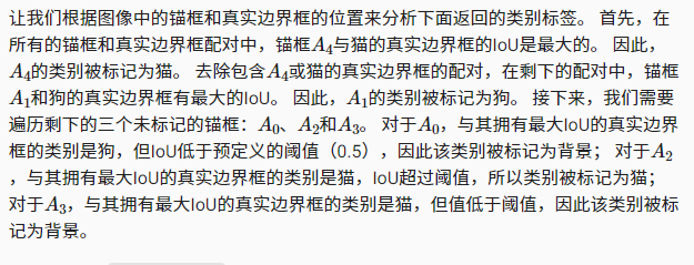
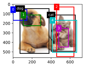
- 一个例子
使用上面定义的multibox_target函数,我们可以根据狗和猫的真实边界框,标注这些锚框的分类和偏移量。
ground_truth = torch.tensor([[0, 0.1, 0.08, 0.52, 0.92],
                         [1, 0.55, 0.2, 0.9, 0.88]])
anchors = torch.tensor([[0, 0.1, 0.2, 0.3], [0.15, 0.2, 0.4, 0.4],
                    [0.63, 0.05, 0.88, 0.98], [0.66, 0.45, 0.8, 0.8],
                    [0.57, 0.3, 0.92, 0.9]])

fig = d2l.plt.imshow(img)
show_bboxes(fig.axes, ground_truth[:, 1:] * bbox_scale, ['dog', 'cat'], 'k')
show_bboxes(fig.axes, anchors * bbox_scale, ['0', '1', '2', '3', '4']);

labels = multibox_target(anchors.unsqueeze(dim=0),
                         ground_truth.unsqueeze(dim=0))
使用非极大值抑制预测边界框
在预测时,我们先为图像生成多个锚框,再为这些锚框一一预测类别和偏移量。 一个预测好的边界框则根据其中某个带有预测偏移量的锚框而生成。 下面我们实现了offset_inverse函数,该函数将锚框和偏移量预测作为输入,并应用逆偏移变换来返回预测的边界框坐标。
#@save
def offset_inverse(anchors, offset_preds):
    """根据带有预测偏移量的锚框来预测边界框"""
    anc = d2l.box_corner_to_center(anchors)
    pred_bbox_xy = (offset_preds[:, :2] * anc[:, 2:] / 10) + anc[:, :2]
    pred_bbox_wh = torch.exp(offset_preds[:, 2:] / 5) * anc[:, 2:]
    pred_bbox = torch.cat((pred_bbox_xy, pred_bbox_wh), axis=1)
    predicted_bbox = d2l.box_center_to_corner(pred_bbox)
    return predicted_bbox
当有许多锚框时,可能会输出许多相似的具有明显重叠的预测边界框,都围绕着同一目标。 为了简化输出,我们可以使用非极大值抑制(non-maximum suppression,NMS)合并属于同一目标的类似的预测边界框。
原理: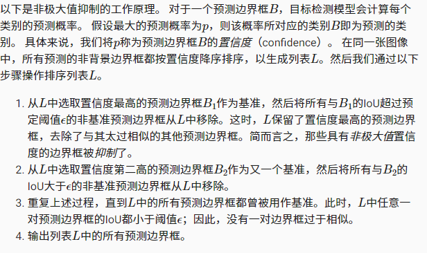
#@save
def nms(boxes, scores, iou_threshold):
    """对预测边界框的置信度进行排序"""
    B = torch.argsort(scores, dim=-1, descending=True)
    keep = []  # 保留预测边界框的指标
    while B.numel() > 0:
        i = B[0]
        keep.append(i)
        if B.numel() == 1: break
        iou = box_iou(boxes[i, :].reshape(-1, 4),
                      boxes[B[1:], :].reshape(-1, 4)).reshape(-1)
        inds = torch.nonzero(iou <= iou_threshold).reshape(-1)
        B = B[inds + 1]
    return torch.tensor(keep, device=boxes.device)
#@save
def multibox_detection(cls_probs, offset_preds, anchors, nms_threshold=0.5,
                       pos_threshold=0.009999999):
    """使用非极大值抑制来预测边界框"""
    device, batch_size = cls_probs.device, cls_probs.shape[0]
    anchors = anchors.squeeze(0)
    num_classes, num_anchors = cls_probs.shape[1], cls_probs.shape[2]
    out = []
    for i in range(batch_size):
        cls_prob, offset_pred = cls_probs[i], offset_preds[i].reshape(-1, 4)
        conf, class_id = torch.max(cls_prob[1:], 0)
        predicted_bb = offset_inverse(anchors, offset_pred)
        keep = nms(predicted_bb, conf, nms_threshold)

        # 找到所有的non_keep索引,并将类设置为背景
        all_idx = torch.arange(num_anchors, dtype=torch.long, device=device)
        combined = torch.cat((keep, all_idx))
        uniques, counts = combined.unique(return_counts=True)
        non_keep = uniques[counts == 1]
        all_id_sorted = torch.cat((keep, non_keep))
        class_id[non_keep] = -1
        class_id = class_id[all_id_sorted]
        conf, predicted_bb = conf[all_id_sorted], predicted_bb[all_id_sorted]
        # pos_threshold是一个用于非背景预测的阈值
        below_min_idx = (conf < pos_threshold)
        class_id[below_min_idx] = -1
        conf[below_min_idx] = 1 - conf[below_min_idx]
        pred_info = torch.cat((class_id.unsqueeze(1),
                               conf.unsqueeze(1),
                               predicted_bb), dim=1)
        out.append(pred_info)
    return torch.stack(out)
anchors = torch.tensor([[0.1, 0.08, 0.52, 0.92], [0.08, 0.2, 0.56, 0.95],
[0.15, 0.3, 0.62, 0.91], [0.55, 0.2, 0.9, 0.88]])
offset_preds = torch.tensor([0] * anchors.numel())
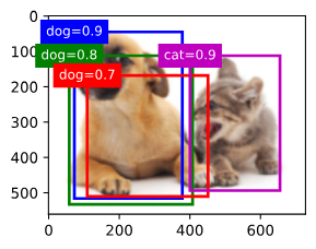
cls_probs = torch.tensor([[0] * 4, # 背景的预测概率
[0.9, 0.8, 0.7, 0.1], # 狗的预测概率
[0.1, 0.2, 0.3, 0.9]]) # 猫的预测概率
fig = d2l.plt.imshow(img)
show_bboxes(fig.axes, anchors * bbox_scale,
['dog=0.9', 'dog=0.8', 'dog=0.7', 'cat=0.9'])
现在我们可以调用multibox_detection函数来执行非极大值抑制,其中阈值设置为0.5。 请注意,我们在示例的张量输入中添加了维度。
我们可以看到返回结果的形状是(批量大小,锚框的数量,6)。 最内层维度中的六个元素提供了同一预测边界框的输出信息。 第一个元素是预测的类索引,从0开始(0代表狗,1代表猫),值-1表示背景或在非极大值抑制中被移除了。 第二个元素是预测的边界框的置信度。 其余四个元素分别是预测边界框左上角和右下角的(x,y)轴坐标(范围介于0和1之间)。
output = multibox_detection(cls_probs.unsqueeze(dim=0),
                            offset_preds.unsqueeze(dim=0),
                            anchors.unsqueeze(dim=0),
                            nms_threshold=0.5)
output
删除-1类别(背景)的预测边界框后,我们可以输出由非极大值抑制保存的最终预测边界框。
fig = d2l.plt.imshow(img)
for i in output[0].detach().numpy():
    if i[0] == -1:
        continue
    label = ('dog=', 'cat=')[int(i[0])] + str(i[1])
    show_bboxes(fig.axes, [torch.tensor(i[2:]) * bbox_scale], label)
实践中,在执行非极大值抑制前,我们甚至可以将置信度较低的预测边界框移除,从而减少此算法中的计算量。 我们也可以对非极大值抑制的输出结果进行后处理。例如,只保留置信度更高的结果作为最终输出。
目标检测数据集
为了快速测试目标检测模型,我们收集并标记了一个小型数据集。 首先,我们拍摄了一组香蕉的照片,并生成了1000张不同角度和大小的香蕉图像。 然后,我们在一些背景图片的随机位置上放一张香蕉的图像。 最后,我们在图片上为这些香蕉标记了边界框。
下载数据集
%matplotlib inline
import os
import pandas as pd
import torch
import torchvision
from d2l import torch as d2l

#@save
d2l.DATA_HUB['banana-detection'] = (
    d2l.DATA_URL + 'banana-detection.zip',
    '5de26c8fce5ccdea9f91267273464dc968d20d72')
读取数据集
#@save
def read_data_bananas(is_train=True):
    """读取香蕉检测数据集中的图像和标签"""
    data_dir = d2l.download_extract('banana-detection')
    csv_fname = os.path.join(data_dir, 'bananas_train' if is_train
                             else 'bananas_val', 'label.csv')
    csv_data = pd.read_csv(csv_fname)
    csv_data = csv_data.set_index('img_name')
    images, targets = [], []
    for img_name, target in csv_data.iterrows():
        images.append(torchvision.io.read_image(
            os.path.join(data_dir, 'bananas_train' if is_train else
                         'bananas_val', 'images', f'{img_name}')))
        # 这里的target包含(类别,左上角x,左上角y,右下角x,右下角y),
        # 其中所有图像都具有相同的香蕉类(索引为0)
        targets.append(list(target))
    return images, torch.tensor(targets).unsqueeze(1) / 256
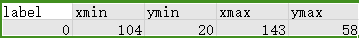
标签文件:
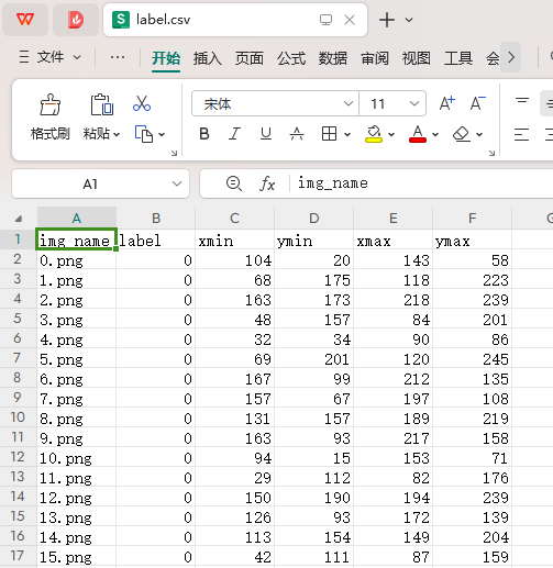
读取数据集,图像的小批量的形状为(批量大小、通道数、高度、宽度),标签的小批量的形状为(批量大小,m,5),其中m是数据集的任何图像中边界框可能出现的最大数量.通常来说,图像可能拥有不同数量个边界框;因此,在达到m之前,边界框少于m的图像将被非法边界框填充。 这样,每个边界框的标签将被长度为5的数组表示。 数组中的第一个元素是边界框中对象的类别,其中-1表示用于填充的非法边界框。
#@save
class BananasDataset(torch.utils.data.Dataset):
    """一个用于加载香蕉检测数据集的自定义数据集"""
    def __init__(self, is_train):
        self.features, self.labels = read_data_bananas(is_train)
        print('read ' + str(len(self.features)) + (f' training examples' if
              is_train else f' validation examples'))

    def __getitem__(self, idx):
        return (self.features[idx].float(), self.labels[idx])

    def __len__(self):
        return len(self.features)


#@save
def load_data_bananas(batch_size):
    """加载香蕉检测数据集"""
    train_iter = torch.utils.data.DataLoader(BananasDataset(is_train=True),
                                             batch_size, shuffle=True)
    val_iter = torch.utils.data.DataLoader(BananasDataset(is_train=False),
                                           batch_size)
    return train_iter, val_iter
batch_size, edge_size = 32, 256
train_iter, _ = load_data_bananas(batch_size)
batch = next(iter(train_iter))
batch[0].shape, batch[1].shape
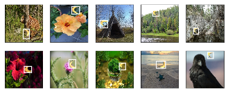
测试图片
imgs = (batch[0][0:10].permute(0, 2, 3, 1)) / 255
axes = d2l.show_images(imgs, 2, 5, scale=2)
for ax, label in zip(axes, batch[1][0:10]):
    d2l.show_bboxes(ax, [label[0][1:5] * edge_size], colors=['w'])
多尺度目标检测
多尺度锚框
如果每个像素都生成锚框,最终可能生成太多锚框需要计算,为了减少锚框数量,不同尺度下,可以生成不同大小和数量的锚框。用较小的锚框检测较小的物体时,可以采样更多的区域,对于较大的物体,则可以采样较小的区域。
锚框中的(x,y)轴坐标值已经被除以特则会概念图的宽度和高度,因此这些值介于0-1之间,可以表示特征图中锚框的相对位置。
以下函数将均匀地对任何输入图像中fmap_h行和fmap_w列中的像素进行采样(采样数量为fmap_hfmap_w)。 以这些均匀采样的像素为中心,将会生成大小为s(大小为图像高宽s)且宽高比(ratios)不同的锚框
%matplotlib inline
import torch
from d2l import torch as d2l

img = d2l.plt.imread('../img/catdog.jpg')
h, w = img.shape[:2]
h, w
def display_anchors(fmap_w, fmap_h, s):
    d2l.set_figsize()
    # 前两个维度上的值不影响输出
    fmap = torch.zeros((1, 10, fmap_h, fmap_w))
    anchors = d2l.multibox_prior(fmap, sizes=s, ratios=[1, 2, 0.5])
    bbox_scale = torch.tensor((w, h, w, h))
    d2l.show_bboxes(d2l.plt.imshow(img).axes,
                    anchors[0] * bbox_scale)
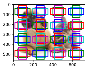
测试函数,锚框的尺度设置为0.15,特征图的高度和宽度设置为4。
display_anchors(fmap_w=4, fmap_h=4, s=[0.15])
多尺度检测
我们用输入图像在某个感受野区域内的信息,来预测输入图像上与该区域位置相近的锚框类别和偏移量。
当不同层的特征图在输入图像上分别拥有不同大小的感受野时,它们可以用于检测不同大小的目标。
利用深层神经网络在多个层次上对图像进行分层表示,从而实现多尺度目标检测。
单发多框检测(SSD)
用的比较多的目标检测模型
用卷积神经网抽取图片特征,,生成很多 框,对每个 判断是不是有目标物体,同时回归看真正的边界框在哪,再卷积(减半模块)
模型

模型主要由基础网络组成,其后是几个多尺度特征块。
基本网络用于从输入图像中提取特征,因此它可以使用深度卷积神经网络。 VGG,ResNet。可以设计基础网络,使它输出的高和宽较大。 这样一来,基于该特征图生成的锚框数量较多,可以用来检测尺寸较小的目标。 接下来的每个多尺度特征块将上一层提供的特征图的高和宽缩小(如减半),并使特征图中每个单元在输入图像上的感受野变得更广阔。
类别预测层
设目标类别的数量为q。这样一来,锚框有q+1个类别,其中0类是背景。
%matplotlib inline
import torch
import torchvision
from torch import nn
from torch.nn import functional as F
from d2l import torch as d2l


def cls_predictor(num_inputs, num_anchors, num_classes):
    return nn.Conv2d(num_inputs, num_anchors * (num_classes + 1),
                     kernel_size=3, padding=1)
边界框预测层
def bbox_predictor(num_inputs, num_anchors):
    return nn.Conv2d(num_inputs, num_anchors * 4, kernel_size=3, padding=1)
连结多尺度的预测
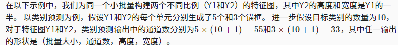
单发多框检测使用多尺度特征图来生成锚框并预测其类别和偏移量。 在不同的尺度下,特征图的形状或以同一单元为中心的锚框的数量可能会有所不同。 因此,不同尺度下预测输出的形状可能会有所不同。
def forward(x, block):
    return block(x)

Y1 = forward(torch.zeros((2, 8, 20, 20)), cls_predictor(8, 5, 10))
Y2 = forward(torch.zeros((2, 16, 10, 10)), cls_predictor(16, 3, 10))
Y1.shape, Y2.shape
正如我们所看到的,除了批量大小这一维度外,其他三个维度都具有不同的尺寸。 为了将这两个预测输出链接起来以提高计算效率,我们将把这些张量转换为更一致的格式。
通道维包含中心相同的锚框的预测结果。我们首先将通道维移到最后一维。 因为不同尺度下批量大小仍保持不变,我们可以将预测结果转成二维的(批量大小,高宽通道数)的格式,以方便之后在维度1上的连结。
def flatten_pred(pred):
    return torch.flatten(pred.permute(0, 2, 3, 1), start_dim=1)

def concat_preds(preds):
    return torch.cat([flatten_pred(p) for p in preds], dim=1)
高和宽减半块
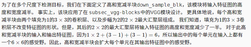
def down_sample_blk(in_channels, out_channels):
    blk = []
    for _ in range(2):
        blk.append(nn.Conv2d(in_channels, out_channels,
                             kernel_size=3, padding=1))
        blk.append(nn.BatchNorm2d(out_channels))
        blk.append(nn.ReLU())
        in_channels = out_channels
    blk.append(nn.MaxPool2d(2))
    return nn.Sequential(*blk)
forward(torch.zeros((2, 3, 20, 20)), down_sample_blk(3, 10)).shape
torch.Size([2, 10, 10, 10])
基本网络块
基本网络块用于从输入图像中抽取特征。 为了计算简洁,我们构造了一个小的基础网络,该网络串联3个高和宽减半块,并逐步将通道数翻倍。
def base_net():
    blk = []
    num_filters = [3, 16, 32, 64]
    for i in range(len(num_filters) - 1):
        blk.append(down_sample_blk(num_filters[i], num_filters[i+1]))
    return nn.Sequential(*blk)

forward(torch.zeros((2, 3, 256, 256)), base_net()).shape
给定输入图像的形状为256256,此基本网络块输出的特征图形状为
(3232)。
完整的模型
完整的单发多框检测模型由五个模块组成。每个块生成的特征图既用于生成锚框,又用于预测这些锚框的类别和偏移量。在这五个模块中,第一个是基本网络块,第二个到第四个是高和宽减半块,最后一个模块使用全局最大池将高度和宽度都降到1。从技术上讲,第二到第五个区块都是 图13.7.1中的多尺度特征块。
def get_blk(i):
    if i == 0:
        blk = base_net()
    elif i == 1:
        blk = down_sample_blk(64, 128)
    elif i == 4:
        blk = nn.AdaptiveMaxPool2d((1,1))
    else:
        blk = down_sample_blk(128, 128)
    return blk
现在我们为每个块定义前向传播。与图像分类任务不同,此处的输出包括:CNN特征图Y;在当前尺度下根据Y生成的锚框;预测的这些锚框的类别和偏移量(基于Y)。
def blk_forward(X, blk, size, ratio, cls_predictor, bbox_predictor):
    Y = blk(X)
    anchors = d2l.multibox_prior(Y, sizes=size, ratios=ratio)
    cls_preds = cls_predictor(Y)
    bbox_preds = bbox_predictor(Y)
    return (Y, anchors, cls_preds, bbox_preds)
sizes = [[0.2, 0.272], [0.37, 0.447], [0.54, 0.619], [0.71, 0.79],
         [0.88, 0.961]]
ratios = [[1, 2, 0.5]] * 5
num_anchors = len(sizes[0]) + len(ratios[0]) - 1
class TinySSD(nn.Module):
    def __init__(self, num_classes, **kwargs):
        super(TinySSD, self).__init__(**kwargs)
        self.num_classes = num_classes
        idx_to_in_channels = [64, 128, 128, 128, 128]
        for i in range(5):
            # 即赋值语句self.blk_i=get_blk(i)
            setattr(self, f'blk_{i}', get_blk(i))
            setattr(self, f'cls_{i}', cls_predictor(idx_to_in_channels[i],
                                                    num_anchors, num_classes))
            setattr(self, f'bbox_{i}', bbox_predictor(idx_to_in_channels[i],
                                                      num_anchors))

    def forward(self, X):
        anchors, cls_preds, bbox_preds = [None] * 5, [None] * 5, [None] * 5
        for i in range(5):
            # getattr(self,'blk_%d'%i)即访问self.blk_i
            X, anchors[i], cls_preds[i], bbox_preds[i] = blk_forward(
                X, getattr(self, f'blk_{i}'), sizes[i], ratios[i],
                getattr(self, f'cls_{i}'), getattr(self, f'bbox_{i}'))
        anchors = torch.cat(anchors, dim=1)
        cls_preds = concat_preds(cls_preds)
        cls_preds = cls_preds.reshape(
            cls_preds.shape[0], -1, self.num_classes + 1)
        bbox_preds = concat_preds(bbox_preds)
        return anchors, cls_preds, bbox_preds

net = TinySSD(num_classes=1)
X = torch.zeros((32, 3, 256, 256))
anchors, cls_preds, bbox_preds = net(X)

print('output anchors:', anchors.shape)
print('output class preds:', cls_preds.shape)
print('output bbox preds:', bbox_preds.shape)
训练模型
读取数据集和初始化
batch_size = 32
train_iter, _ = d2l.load_data_bananas(batch_size)
device, net = d2l.try_gpu(), TinySSD(num_classes=1)
trainer = torch.optim.SGD(net.parameters(), lr=0.2, weight_decay=5e-4)
定义损失函数和评价函数
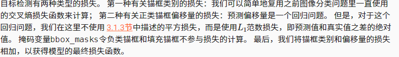
cls_loss = nn.CrossEntropyLoss(reduction='none')
bbox_loss = nn.L1Loss(reduction='none')

def calc_loss(cls_preds, cls_labels, bbox_preds, bbox_labels, bbox_masks):
    batch_size, num_classes = cls_preds.shape[0], cls_preds.shape[2]
    cls = cls_loss(cls_preds.reshape(-1, num_classes),
                   cls_labels.reshape(-1)).reshape(batch_size, -1).mean(dim=1)
    bbox = bbox_loss(bbox_preds * bbox_masks,
                     bbox_labels * bbox_masks).mean(dim=1)
    return cls + bbox
def cls_eval(cls_preds, cls_labels):
    # 由于类别预测结果放在最后一维,argmax需要指定最后一维。
    return float((cls_preds.argmax(dim=-1).type(
        cls_labels.dtype) == cls_labels).sum())

def bbox_eval(bbox_preds, bbox_labels, bbox_masks):
    return float((torch.abs((bbox_labels - bbox_preds) * bbox_masks)).sum())
训练模型
num_epochs, timer = 20, d2l.Timer()
animator = d2l.Animator(xlabel='epoch', xlim=[1, num_epochs],
                        legend=['class error', 'bbox mae'])
net = net.to(device)
for epoch in range(num_epochs):
    # 训练精确度的和,训练精确度的和中的示例数
    # 绝对误差的和,绝对误差的和中的示例数
    metric = d2l.Accumulator(4)
    net.train()
    for features, target in train_iter:
        timer.start()
        trainer.zero_grad()
        X, Y = features.to(device), target.to(device)
        # 生成多尺度的锚框,为每个锚框预测类别和偏移量
        anchors, cls_preds, bbox_preds = net(X)
        # 为每个锚框标注类别和偏移量
        bbox_labels, bbox_masks, cls_labels = d2l.multibox_target(anchors, Y)
        # 根据类别和偏移量的预测和标注值计算损失函数
        l = calc_loss(cls_preds, cls_labels, bbox_preds, bbox_labels,
                      bbox_masks)
        l.mean().backward()
        trainer.step()
        metric.add(cls_eval(cls_preds, cls_labels), cls_labels.numel(),
                   bbox_eval(bbox_preds, bbox_labels, bbox_masks),
                   bbox_labels.numel())
    cls_err, bbox_mae = 1 - metric[0] / metric[1], metric[2] / metric[3]
    animator.add(epoch + 1, (cls_err, bbox_mae))
print(f'class err {cls_err:.2e}, bbox mae {bbox_mae:.2e}')
print(f'{len(train_iter.dataset) / timer.stop():.1f} examples/sec on '
      f'{str(device)}')
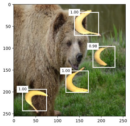
预测目标
我们希望能把图像里面所有我们感兴趣的目标检测出来。在下面,我们读取并调整测试图像的大小,然后将其转成卷积层需要的四维格式。
X = torchvision.io.read_image('../img/banana.jpg').unsqueeze(0).float()
img = X.squeeze(0).permute(1, 2, 0).long()
使用下面的multibox_detection函数,我们可以根据锚框及其预测偏移量得到预测边界框。然后,通过非极大值抑制来移除相似的预测边界框。
def predict(X):
    net.eval()
    anchors, cls_preds, bbox_preds = net(X.to(device))
    cls_probs = F.softmax(cls_preds, dim=2).permute(0, 2, 1)
    output = d2l.multibox_detection(cls_probs, bbox_preds, anchors)
    idx = [i for i, row in enumerate(output[0]) if row[0] != -1]
    return output[0, idx]

output = predict(X)
def display(img, output, threshold):
    d2l.set_figsize((5, 5))
    fig = d2l.plt.imshow(img)
    for row in output:
        score = float(row[1])
        if score < threshold:
            continue
        h, w = img.shape[0:2]
        bbox = [row[2:6] * torch.tensor((w, h, w, h), device=row.device)]
        d2l.show_bboxes(fig.axes, bbox, '%.2f' % score, 'w')

display(img, output.cpu(), threshold=0.9)