逻辑回归(机器学习)

2024-07-17 13:12:01
开发
20

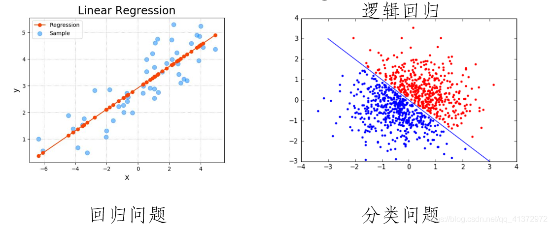
上一题篇文章写了线性回归以及梯度下降法，这篇文章讲一下逻辑回归。虽然它叫逻辑回归，但是它并非回归模型，而是一个分类模型。那么回归和分类有什么区别呢？在上一篇文章中，我们以住房各特征预测了房价中位数。这个是给定数据，预测一个连续的数据。而分类呢？还是举出上面的例子，只不过这次我不需要预测价格中位数了，只需要预测这个房子的“好与坏”，值域只有（好、坏）。

最后注意：

求导后是

$\frac{\partial J(\theta)}{\partial \theta_{j}}=\frac{1}{m}\sum_{i=1}^{m}(h_{\theta}(x^{(i)})-y^{(i)})x^{(i)}_{j}$

矩阵形式是：
$\frac{\partial J(\theta)}{\partial \theta}=\frac{1}{m}X^{T}(g(X\theta )-y)$

下面是逻辑回归矩阵形式的推导：

实验操作：
要求：已知有数据（exam1,exam2,aeecpted），第一个和第二个是成绩，第三个是是否被大学录取，要求根据成绩来预测是否被大学录取。

直接给出数据，自己复制到txt中测试(数据在最后面)：

第一步先看一下数据可视化：

import pandas as pd
import numpy as np
import matplotlib

matplotlib.use('tKAgg')
import matplotlib.pyplot as plt

path = "D:\JD\Documents\大学等等等\自学部分\machine_-learning-master\machine_-learning-master\ex_2\ex2data1.txt"
data = pd.read_csv(path, names=['Exam1', 'Exam2', 'Accepted'])
print(data.head())
fig, ax = plt.subplots()
ax.scatter(data[data['Accepted'] == 0]['Exam1'], data[data['Accepted'] == 0]['Exam2'], c='r', marker='x', label='y=0')
ax.scatter(data[data['Accepted'] == 1]['Exam1'], data[data['Accepted'] == 1]['Exam2'], c='g', marker='o', label='y=1')
ax.legend()
ax.set(
    xlabel='exam1',
    ylabel='exam2'
)
plt.show()

接下来写函数：

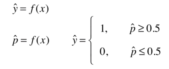
预测值为：

$\hat{y}=g(X\theta)$

这里面代价函数：

$J(\theta)=-\frac{1}{m}[y*log(\hat{y})+(1-y)*log(1-\hat{y})]$

注意矩阵乘法和*乘法最后得到的结果不一样哦！

def get_Xy(data):
    data.insert(0, 'ones', 1)
    X_ = data.iloc[:, :-1]  # 获取除了最后一列的数据集
    y_ = data.iloc[:, -1]  # 获取最后一列的数据集

    X = X_.values  # 转化为数组
    y = y_.values.reshape(len(y_.values), 1)  # 从pandas中取出的只有一维的数据自动是行向量，或者(n,)没有第二维，所以reshape以下称为(n,1)
    return X, y


# sigmoid函数
def sigmoid(z):
    return 1 / (1 + np.exp(-z))

#损失函数
def costFunction(X, y, theta):
    A = sigmoid(X @ theta)  # 预测值一维矩阵
    epsilon = 1e-5  # 用来避免对数计算中的无效值
    first = y * np.log(A + epsilon)  # 转置后直接得到一个数，如果不转置还需要对矩阵求和
    second = (1 - y) * np.log(1 - A + epsilon)
    return -np.sum(first + second) / len(y)

接下来，梯度下降！

上面推导的过程求出来了损失函数求导的结果：
然后对参数进行梯度下降，迭代公式为：

$\theta = \theta - \frac{\alpha }{m}*X^{T}(g(X\theta)-y)$

# 定义梯度下降
def gradientDescent(X, y, theta, iters, alpha):
    m = len(X)
    costs = []
    for i in range(iters):
        A = sigmoid(X @ theta)
        theta = theta - alpha / m * X.T @ (A - y)
        cost = costFunction(X, y, theta)
        costs.append(cost)
        if i % 1000 == 0:
            print(f"Iteration {i}: cost = {cost}")
    return costs, theta

下面是损失函数随着迭代次数值的变化：

最后的theta是[[-23.77498778]，[ 0.18690941]，[ 0.18046614]]

实现预测：

def predict(X,theta):
    pre = sigmoid(X@theta)
    return [1 if i >= 0.5 else 0 for i in pre ]

预测值与真实值之间对比：

完整代码：

import pandas as pd
import numpy as np
import matplotlib

matplotlib.use('tKAgg')
import matplotlib.pyplot as plt

# 读取数据
path = "D:\\JD\\Documents\\大学等等等\\自学部分\\machine_-learning-master\\machine_-learning-master\\ex_2\\ex2data1.txt"
data = pd.read_csv(path, names=['Exam1', 'Exam2', 'Accepted'])
print(data.head())

# 绘制散点图
fig, ax = plt.subplots()
ax.scatter(data[data['Accepted'] == 0]['Exam1'], data[data['Accepted'] == 0]['Exam2'], c='r', marker='x', label='y=0')
ax.scatter(data[data['Accepted'] == 1]['Exam1'], data[data['Accepted'] == 1]['Exam2'], c='g', marker='o', label='y=1')
ax.legend()
ax.set(
    xlabel='exam1',
    ylabel='exam2'
)
plt.show()

# 提取X和y
def get_Xy(data):
    data.insert(0, 'ones', 1)
    X_ = data.iloc[:, :-1]  # 获取除了最后一列的数据集
    y_ = data.iloc[:, -1]  # 获取最后一列的数据集

    X = X_.values  # 转化为数组
    y = y_.values.reshape(len(y_.values), 1)  # 从pandas中取出的只有一维的数据自动是行向量，或者(n,)没有第二维，所以reshape以下称为(n,1)
    return X, y

# sigmoid函数
def sigmoid(z):
    return 1 / (1 + np.exp(-z))

# 损失函数
def costFunction(X, y, theta):
    A = sigmoid(X @ theta)  # 预测值一维矩阵
    epsilon = 1e-5  # 用来避免对数计算中的无效值
    first = y * np.log(A + epsilon)  # 转置后直接得到一个数，如果不转置还需要对矩阵求和
    second = (1 - y) * np.log(1 - A + epsilon)
    return -np.sum(first + second) / len(y)

theta = np.zeros((3, 1))
X, y = get_Xy(data)
const_init = costFunction(X, y, theta)
print(const_init)

# 定义梯度下降
def gradientDescent(X, y, theta, iters, alpha):
    m = len(X)
    costs = []
    for i in range(iters):
        A = sigmoid(X @ theta)
        theta = theta - alpha / m * X.T @ (A - y)
        cost = costFunction(X, y, theta)
        costs.append(cost)
        if i % 1000 == 0:
            print(f"Iteration {i}: cost = {cost}")
    return costs, theta

alpha = 0.004
iters = 200000
costs, theta = gradientDescent(X, y, theta, iters, alpha)

print("---------------------------")
print(costs)
print("---------------------------")
print(theta)

plt.figure()
plt.plot(range(iters), costs, label='Cost')
plt.xlabel('Iterations')
plt.ylabel('Cost')
plt.title('Cost Function Convergence')
plt.legend()
plt.show()

print("---------------------------")
# print(costs)
print(theta)

def predict(X,theta):
    pre = sigmoid(X@theta)
    return [1 if i >= 0.5 else 0 for i in pre ]


y_pre = predict(X,theta)

# 绘制真实值与预测值的比较图
plt.figure()
plt.plot(range(len(y)), y, label='real_values', linestyle='-', marker='o', color='g')
plt.plot(range(len(y)), y_pre, label='pre_value', linestyle='--', marker='x', color='r')
plt.xlabel('label')
plt.ylabel('value')
plt.title('differ')
plt.legend()
plt.show()

附：使用数据集

34.62365962451697,78.0246928153624,0
30.28671076822607,43.89499752400101,0
35.84740876993872,72.90219802708364,0
60.18259938620976,86.30855209546826,1
79.0327360507101,75.3443764369103,1
45.08327747668339,56.3163717815305,0
61.10666453684766,96.51142588489624,1
75.02474556738889,46.55401354116538,1
76.09878670226257,87.42056971926803,1
84.43281996120035,43.53339331072109,1
95.86155507093572,38.22527805795094,0
75.01365838958247,30.60326323428011,0
82.30705337399482,76.48196330235604,1
69.36458875970939,97.71869196188608,1
39.53833914367223,76.03681085115882,0
53.9710521485623,89.20735013750205,1
69.07014406283025,52.74046973016765,1
67.94685547711617,46.67857410673128,0
70.66150955499435,92.92713789364831,1
76.97878372747498,47.57596364975532,1
67.37202754570876,42.83843832029179,0
89.67677575072079,65.79936592745237,1
50.534788289883,48.85581152764205,0
34.21206097786789,44.20952859866288,0
77.9240914545704,68.9723599933059,1
62.27101367004632,69.95445795447587,1
80.1901807509566,44.82162893218353,1
93.114388797442,38.80067033713209,0
61.83020602312595,50.25610789244621,0
38.78580379679423,64.99568095539578,0
61.379289447425,72.80788731317097,1
85.40451939411645,57.05198397627122,1
52.10797973193984,63.12762376881715,0
52.04540476831827,69.43286012045222,1
40.23689373545111,71.16774802184875,0
54.63510555424817,52.21388588061123,0
33.91550010906887,98.86943574220611,0
64.17698887494485,80.90806058670817,1
74.78925295941542,41.57341522824434,0
34.1836400264419,75.2377203360134,0
83.90239366249155,56.30804621605327,1
51.54772026906181,46.85629026349976,0
94.44336776917852,65.56892160559052,1
82.36875375713919,40.61825515970618,0
51.04775177128865,45.82270145776001,0
62.22267576120188,52.06099194836679,0
77.19303492601364,70.45820000180959,1
97.77159928000232,86.7278223300282,1
62.07306379667647,96.76882412413983,1
91.56497449807442,88.69629254546599,1
79.94481794066932,74.16311935043758,1
99.2725269292572,60.99903099844988,1
90.54671411399852,43.39060180650027,1
34.52451385320009,60.39634245837173,0
50.2864961189907,49.80453881323059,0
49.58667721632031,59.80895099453265,0
97.64563396007767,68.86157272420604,1
32.57720016809309,95.59854761387875,0
74.24869136721598,69.82457122657193,1
71.79646205863379,78.45356224515052,1
75.3956114656803,85.75993667331619,1
35.28611281526193,47.02051394723416,0
56.25381749711624,39.26147251058019,0
30.05882244669796,49.59297386723685,0
44.66826172480893,66.45008614558913,0
66.56089447242954,41.09209807936973,0
40.45755098375164,97.53518548909936,1
49.07256321908844,51.88321182073966,0
80.27957401466998,92.11606081344084,1
66.74671856944039,60.99139402740988,1
32.72283304060323,43.30717306430063,0
64.0393204150601,78.03168802018232,1
72.34649422579923,96.22759296761404,1
60.45788573918959,73.09499809758037,1
58.84095621726802,75.85844831279042,1
99.82785779692128,72.36925193383885,1
47.26426910848174,88.47586499559782,1
50.45815980285988,75.80985952982456,1
60.45555629271532,42.50840943572217,0
82.22666157785568,42.71987853716458,0
88.9138964166533,69.80378889835472,1
94.83450672430196,45.69430680250754,1
67.31925746917527,66.58935317747915,1
57.23870631569862,59.51428198012956,1
80.36675600171273,90.96014789746954,1
68.46852178591112,85.59430710452014,1
42.0754545384731,78.84478600148043,0
75.47770200533905,90.42453899753964,1
78.63542434898018,96.64742716885644,1
52.34800398794107,60.76950525602592,0
94.09433112516793,77.15910509073893,1
90.44855097096364,87.50879176484702,1
55.48216114069585,35.57070347228866,0
74.49269241843041,84.84513684930135,1
89.84580670720979,45.35828361091658,1
83.48916274498238,48.38028579728175,1
42.2617008099817,87.10385094025457,1
99.31500880510394,68.77540947206617,1
55.34001756003703,64.9319380069486,1
74.77589300092767,89.52981289513276,1

原文地址:https://blog.csdn.net/2303_77275067/article/details/140455330 本文来自互联网用户投稿，该文观点仅代表作者本人，不代表本站立场。本站仅提供信息存储空间服务，不拥有所有权，不承担相关法律责任。如若转载，请注明出处：https://www.suanlizi.com/kf/1813441504308498432.html 如若内容造成侵权/违法违规/事实不符，请联系《酸梨子》网邮箱：1419361763@qq.com进行投诉反馈，一经查实，立即删除！

阅读全部

逻辑回归(机器学习)

相关推荐

最近更新

热门阅读