机器学习：逻辑回归

概念

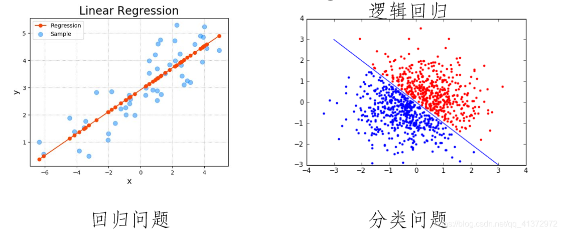
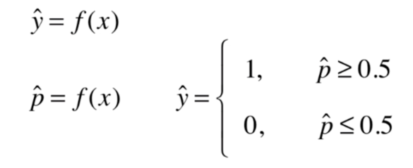
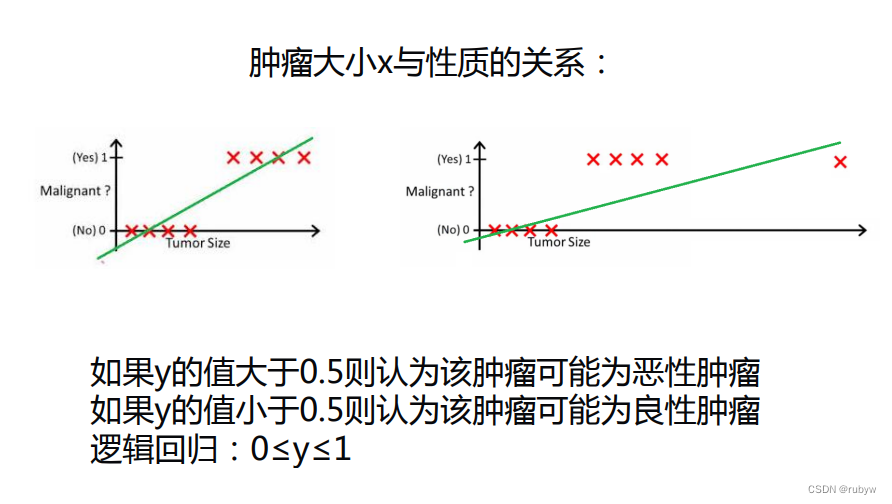
首先，逻辑回归属于分类算法，是线性分类器。我们可以认为逻辑回归是在多元线性回归的基础上把结果给映射到0-1的区间内，hθ（x）越接近1越有可能是正例，反之，越接近0越有可能是负例。那么，我们该通过什么函数把结果映射到0-1之间呢？

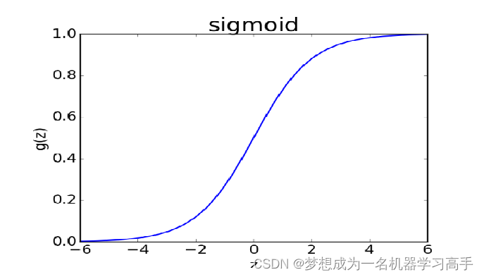
Sigmoid函数

在这里，我们实际上是把作为变量传入，得到

import numpy as np
import math
import matplotlib.pyplot as plt

def sigmoid(x):
    a =[]
    for item in  x:
        a.append(1.0/(1.0+math.exp(-item)))
    return a

x = np.arange(-15,15,0.1)
y = sigmoid(x)

plt.plot(x,y)
plt.show()

这里我设定的自变量范围为[-15,15]，但实际上sigmoid函数定义域为[-inf,+inf]。当自变量为0时，函数值为0.5。

分类器的任务就是找到一个边界，这个边界可以尽可能地划分我们的数据集。当我们把0.5作为边界时，我们要找的就是的解，即θ.TX = 0时θ的值。

广义线性回归

伯努利分布

如果随机变量只能取0和1两个值，则称其服从伯努利分布。

记作

p为正例概率，即当x=1时的概率。但是我们发现这样的分段函数比较难求它的损失函数。为了将分段函数整合，我们先引入广义线性回归的概念。

广义线性回归

当考虑一个分类或者回归问题时，我们就是想预测某个随机变量y,y是某些特征x的函数。为了推广广义线性模式，我们做出三个假设。

一，P(y|(x,θ)) 服从指数族分布。

二，给定x，我们的目的是为了预测T(y)在条件x下的期望，一般情况T(y) = y,这就意味着我们希望预测h(x) = E(y|x)。 

三，参数η和输入x是线性相关的，η=θ.TX

 指数族分布（The Exponential Family Distribution）

指数族分布有：高斯分布，二项分布，伯努利分布，多项分布，泊松分布，指数分布，beta分布，拉普拉斯分布，γ分布。对于回归来说，如果y服从某个指数分布，那么就可以用广义线性回归来建立模型。

通式为

或者

η：自然参数，在线性回归中 

T(y):充分统计量，一般情况下为y

a(η)：对数部分函数，这部分确保分布积分结果为1。

伯努利分布其实也是指数族分布的一种，推导证明：

 在这里，我们成功地将分段函数整合在一个等式中，方便求解后面的损失函数。

φ：正例概率。

y:1或0，正例或负例。

对比

由此可知，

我们发现，这与sigmoid函数推导出来的结果是一致的，这便是逻辑回归使用sigmoid函数的原因。

损失函数推导

我们使用最大似然估计（MLE），根据若干已知的X，y找到一组w使得X作为已知条件下y发生的概率最大。

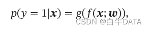
sigmoid(w,x)输出的含义为P(y=1|w,x)，即在w,x条件下正例概率，那么负例概率P(y=0|w,x) = 1-sigmoid(w,x)。

只要让我们的sigmoid(w,x)函数在训练集上预测概率最大，sigmoid(w,x)就是最好的解。

分段函数显然不符合我们的要求，我们将其变形为

我们假设训练样本相互独立，那么似然函数

自然而然，我们两边取对数

这里我们发现，整个过程和线性回归十分相似，首先构造似然函数，再用最大似然估计，最后得到θ更新迭代的等式，只不过这里不是梯度下降，而是梯度上升，习惯上，我们使用梯度下降。

所以损失函数为

梯度下降

我们发现，最终的梯度公式与线性回归很相似，这是因为它们都是广义线性回归中来的，服从的都是指数族分布。

代码实现

from sklearn.datasets import load_breast_cancer
from sklearn.linear_model import LogisticRegression
from sklearn.preprocessing import scale
import numpy as np
import matplotlib.pyplot as plt
from mpl_toolkits.mplot3d import Axes3D

data = load_breast_cancer()
X,y = data['data'][:,:2],data['target']
lr = LogisticRegression(fit_intercept=False)
lr.fit(X,y)
w1 = lr.coef_[0,0]
w2 = lr.coef_[0,1]

def p_theta_function(features,w1,w2):
    z = w1*features[0] + w2*features[1]
    return 1/(1+np.exp(-z))

def loss_function(samples_features,samples_labels,w1,w2):
    result = 0
    for features,label in zip(samples_features,samples_labels):
        p_result = p_theta_function(features,w1,w2)
        loss_result = -1*label*np.log(p_result) - (1-label)*np.log(1-p_result)
        result += loss_result
    return result


w1_space = np.linspace(w1-0.6,w1+0.6,50)
w2_space = np.linspace(w2-0.6,w2+0.6,50)

result1_ = np.array([loss_function(X,y,i,w2)for i in w1_space])
result2_ = np.array([loss_function(X,y,w1,i)for i in w2_space])

fig = plt.figure(figsize=(8,6))
plt.subplot(2,2,1)
plt.plot(w1_space,result1_)
plt.subplot(2,2,2)
plt.plot(w2_space,result2_)

w1_grid,w2_grid = np.meshgrid(w1_space,w2_space)
loss_grid = loss_function(X,y,w1_grid,w2_grid)
plt.subplot(2,2,3)
plt.contour(w1_grid,w2_grid,loss_grid)
plt.subplot(2,2,4)
plt.contour(w1_grid,w2_grid,loss_grid,30)
fig_2 = plt.figure()
ax = fig_2.add_axes(Axes3D(fig_2))
ax.plot_surface(w1_grid, w2_grid, loss_grid, rstride=1, cstride=1, cmap=plt.get_cmap('rainbow'))
ax.contourf(w1_grid, w2_grid, loss_grid,zdir='z', offset=-2, cmap=plt.get_cmap('rainbow'))
print("θ1 = ",w1)
print("θ2 = ",w2)

plt.show()

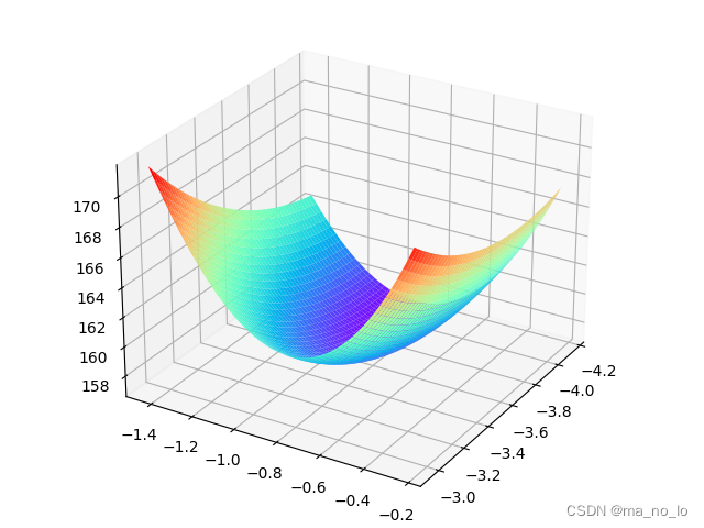
观察图像，我们发现w1,w2两个维度不均匀，等高线组成的是椭圆，在这里，我们使用正则化稍微约束一下。

from sklearn.datasets import load_breast_cancer
from sklearn.linear_model import LogisticRegression
from sklearn.preprocessing import scale
import numpy as np
import matplotlib.pyplot as plt
from mpl_toolkits.mplot3d import Axes3D
data = load_breast_cancer()
X,y = scale(data['data'][:,:2]),data['target']
lr = LogisticRegression(fit_intercept=False)
lr.fit(X,y)
w1 = lr.coef_[0,0]
w2 = lr.coef_[0,1]

def p_theta_function(features,w1,w2):
    z = w1*features[0] + w2*features[1]
    return 1/(1+np.exp(-z))

def loss_function(samples_features,samples_labels,w1,w2):
    result = 0
    for features,label in zip(samples_features,samples_labels):
        p_result = p_theta_function(features,w1,w2)
        loss_result = -1*label*np.log(p_result) - (1-label)*np.log(1-p_result)
        result += loss_result
    return result


w1_space = np.linspace(w1-0.6,w1+0.6,50)
w2_space = np.linspace(w2-0.6,w2+0.6,50)

result1_ = np.array([loss_function(X,y,i,w2)for i in w1_space])
result2_ = np.array([loss_function(X,y,w1,i)for i in w2_space])

fig = plt.figure(figsize=(8,6))
plt.subplot(2,2,1)
plt.plot(w1_space,result1_)
plt.subplot(2,2,2)
plt.plot(w2_space,result2_)

w1_grid,w2_grid = np.meshgrid(w1_space,w2_space)
loss_grid = loss_function(X,y,w1_grid,w2_grid)
plt.subplot(2,2,3)
plt.contour(w1_grid,w2_grid,loss_grid)
plt.subplot(2,2,4)
plt.contour(w1_grid,w2_grid,loss_grid,30)
fig_2 = plt.figure()
ax = fig_2.add_axes(Axes3D(fig_2))
ax.plot_surface(w1_grid, w2_grid, loss_grid, rstride=1, cstride=1, cmap=plt.get_cmap('rainbow'))
ax.contourf(w1_grid, w2_grid, loss_grid,zdir='z', offset=-2, cmap=plt.get_cmap('rainbow'))
print("θ1 = ",w1)
print("θ2 = ",w2)

plt.show()