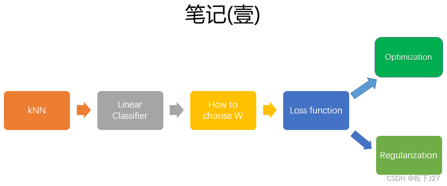
深度学习 --- stanford cs231 编程作业(assignment1，Q2: SVM分类器)

stanford cs231 编程作业之SVM分类器

写在最前面：

深度学习，或者是广义上的任何学习，都是“行千里路”胜过“读万卷书”的学识。这两天光是学了斯坦福cs231n的一些基础理论，越往后学越觉得没什么。但听的云里雾里的地方也越来越多。昨天无意中在这门课的官网上无意中看到了对应的assignments。里面的问题和code都设计的极好！自己在做作业的时候，也才真的认识到“纸上得来终觉浅，绝知此事要躬行。”此言不虚。下面是我自己作业的相关笔记，为了记录也为了分享。

作业相关的code可从这里下载：

Assignment 1

相应的安装方法官网上有详细说明，我自己这里也写了一篇安装说明：

深度学习 --- stanford cs231 编程作业(如何在chrome中安装Google colab）-CSDN博客

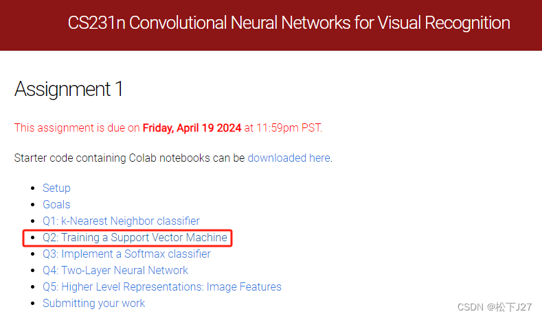
1，这个作业想让我们做什么？

Todo list:

下面我结合代码逐一作出说明。

2，assignment coding --- CIFAR-10数据集

2，1，配置环境，sync Google Drive with Google Colab

# This mounts your Google Drive to the Colab VM.
from google.colab import drive
drive.mount('/content/drive')

# TODO: Enter the foldername in your Drive where you have saved the unzipped
# assignment folder, e.g. 'cs231n/assignments/assignment1/'
FOLDERNAME = 'google colab/cs231/assignments/assignment1/'
assert FOLDERNAME is not None, "[!] Enter the foldername."

# Now that we've mounted your Drive, this ensures that
# the Python interpreter of the Colab VM can load
# python files from within it.
import sys
sys.path.append('/content/drive/My Drive/{}'.format(FOLDERNAME))

# This downloads the CIFAR-10 dataset to your Drive
# if it doesn't already exist.
%cd /content/drive/My\ Drive/$FOLDERNAME/cs231n/datasets/
!bash get_datasets.sh
%cd /content/drive/My\ Drive/$FOLDERNAME

后面为了debug我在这里加了ipdb。

!pip install ipdb
import ipdb

这里load了几个常用的库numpy和matplotlib，值得一提的是专门load了一个保存在“cs231n”目录下的“data_utils.py”文件中的名叫“load_CIFAR10”的函数。

# Run some setup code for this notebook.
import random
import numpy as np
from cs231n.data_utils import load_CIFAR10
import matplotlib.pyplot as plt

# This is a bit of magic to make matplotlib figures appear inline in the
# notebook rather than in a new window.
%matplotlib inline
plt.rcParams['figure.figsize'] = (10.0, 8.0) # set default size of plots
plt.rcParams['image.interpolation'] = 'nearest'
plt.rcParams['image.cmap'] = 'gray'

# Some more magic so that the notebook will reload external python modules;
# see http://stackoverflow.com/questions/1907993/autoreload-of-modules-in-ipython
%load_ext autoreload
%autoreload 2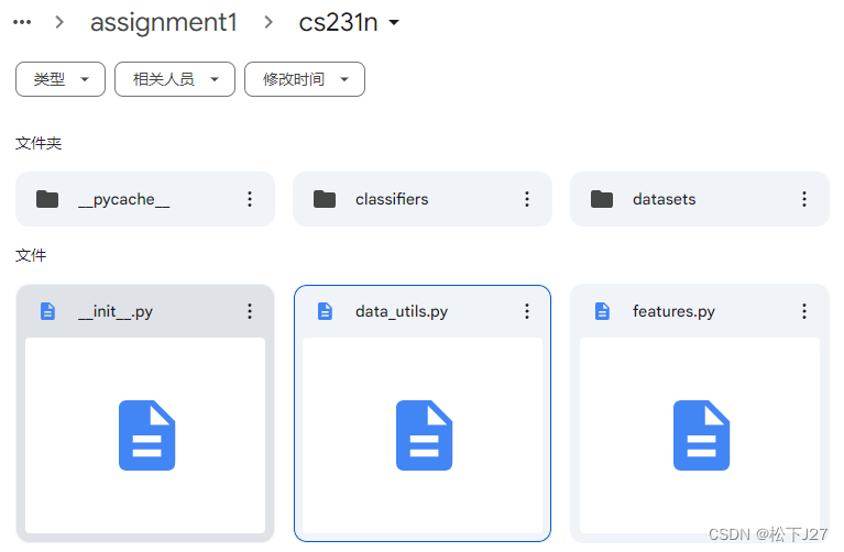

2，2，Load Data

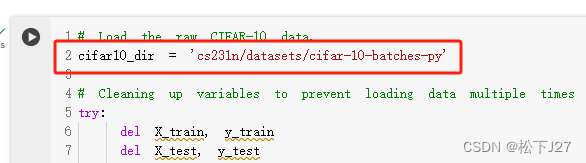
# Load the raw CIFAR-10 data.
cifar10_dir = 'cs231n/datasets/cifar-10-batches-py'

# Cleaning up variables to prevent loading data multiple times (which may cause memory issue)
try:
   del X_train, y_train
   del X_test, y_test
   print('Clear previously loaded data.')
except:
   pass

X_train, y_train, X_test, y_test = load_CIFAR10(cifar10_dir)

# As a sanity check, we print out the size of the training and test data.
print('Training data shape: ', X_train.shape)
print('Training labels shape: ', y_train.shape)
print('Test data shape: ', X_test.shape)
print('Test labels shape: ', y_test.shape)

load CIFAR-10数据（保存在'cs231n/datasets/cifar-10-batches-py'），并且用到了上面的那个函数“load_CIFAR10”。

这里面有个read me，里面是个网站。

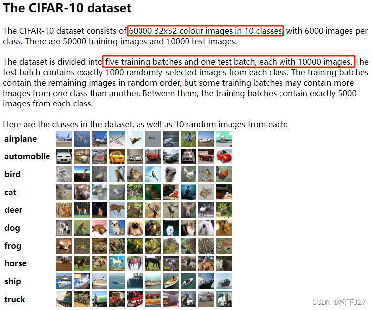
CIFAR-10 and CIFAR-100 datasets

网站上有关于CIFAR-10数据库的说明：

首先，这个数据集是由Alex Krizhevsky(好像他就是著名的AlexNet的作者), Vinod Nair, and Geoffrey Hinton这三个人收集起来的。

CIFAR-10总共有60000张32x32个像素的小图，包含10个种类，每一类都有6000张，共60000张。其中，50000张可专门用于训练模型，即，训练组。另外10000张用于测试训练好的模型，它通过在每个类别中随机选出的1000张图像组成，共10*1000=10000张，即，测试组。

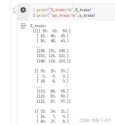
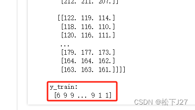
根据输出的结果来看，变量X_train, y_train, X_test, y_test中保存数组的尺寸和官方的说明一致。共50000个数据for train，10000个数据for test。其中，X_train和X_test保存的是彩色图像。而y_train和y_test，保存的是这些图像所对应的种类（0~9之间的一个数）。（下面的这段print是我自己加的。）

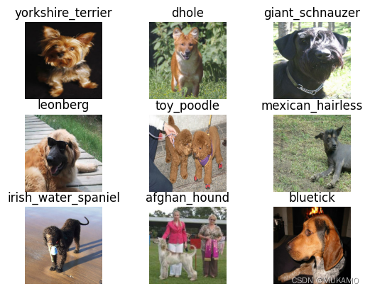
2，3，Data visualize数据的可视化

# Visualize some examples from the dataset.
# We show a few examples of training images from each class.
classes = ['plane', 'car', 'bird', 'cat', 'deer', 'dog', 'frog', 'horse', 'ship', 'truck']
num_classes = len(classes)
samples_per_class = 7
#遍历classes数组，其中y返回的是数组classes的索引,cls返回的是数组classes的Data。例如y=0,cls='plane'.
for y, cls in enumerate(classes):
    #在y_train数组中找出所有等于y的元素，并保存到idxs中
    idxs = np.flatnonzero(y_train == y)
    #在idxs中随机选择7个元素，保存到idxs中
    idxs = np.random.choice(idxs, samples_per_class, replace=False)
    #遍历idxs数组，其中i返回的是数组idxs的索引,idx返回的是数组idxs所保存的内容。例如y=0,idx=35628.
    for i, idx in enumerate(idxs):
        plt_idx = i * num_classes + y + 1
        plt.subplot(samples_per_class, num_classes, plt_idx)
        plt.imshow(X_train[idx].astype('uint8'))
        plt.axis('off')
        if i == 0:
            plt.title(cls)
plt.show()

这些代码是官方写好的，我这里只是大概介绍一下。这段代码主要实现了两个功能，其中上部分代码是在选图。

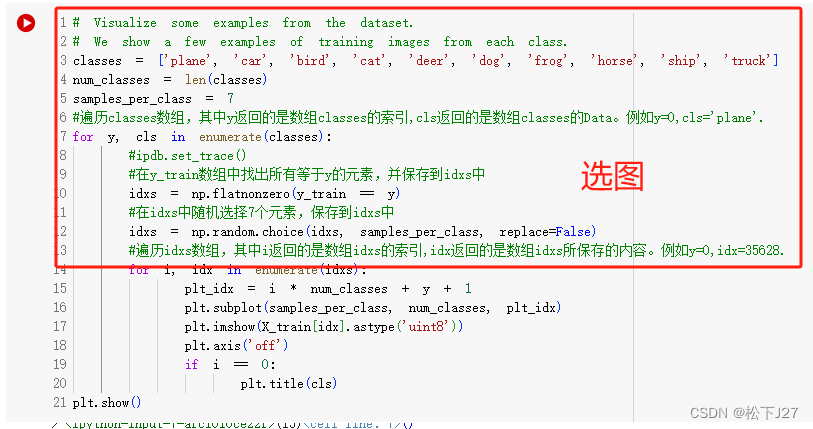
大意就是先找到某一类图像在y_train中所有的位置。例如在下图的debug信息中，当y=0时，(对应的cls="plane")函数np.flatnonzero汇总了5000个lable=y=0的图像在y_train中的位置信息并返回给idxs。

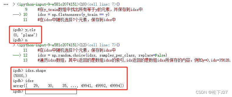
接下来，在idxs所保存的5000个“第0类”图像中随机选出了7个。

这一第一部分的工作，下面的工作就是画图了。遍历上一步保存在数组“idxs”中的7张图，并通过subplot的方式画在同一个figure里。其中，对plt.subplot(samples_per_class, num_classes, plt_idx) 而言：samples_per_class(表示每个类的样本数)是行数，num_classes(表示类别数) 是列数，plt_idx 是子图的位置。

因此，就本例而言共有10个类别，每个类别显示7个样本，总共有70个子图，它们将被排列在一个7行10列的网格中。

得到如下结果（这里每个人的运行结果都可能不一样，因为他是随机抽取的）：

2，4，分配数据集

# Split the data into train, val, and test sets. In addition we will
# create a small development set as a subset of the training data;
# we can use this for development so our code runs faster.
num_training = 49000
num_validation = 1000
num_test = 1000
num_dev = 500

#ipdb.set_trace()

# Our validation set(验证集) will be num_validation points from the original
# training set.
mask = range(num_training, num_training + num_validation)
X_val = X_train[mask]
y_val = y_train[mask]

# Our training set(训练集) will be the first num_train points from the original
# training set.
mask = range(num_training)
X_train = X_train[mask]
y_train = y_train[mask]

# 用于开发的样本子集
# We will also make a development set(开发集), which is a small subset of
# the training set.
'''
np.random.choice：函数用于从一个给定的一维数组中随机采样。参数 replace 控制采样时是否允许重复。
当 replace=True 时，采样是有放回的；当 replace=False 时，采样是无放回的。

具体来说：
replace=True：允许重复采样，即每次从数组中随机选择一个元素，选择后该元素依然可以被再次选择。
这样可能会出现相同的元素被多次选择的情况。
replace=False：不允许重复采样，即每次从数组中随机选择一个元素，选择后该元素会被移除，不再参与后续的采样。
这样每个元素只会被选择一次。
'''
mask = np.random.choice(num_training, num_dev, replace=False)
X_dev = X_train[mask]
y_dev = y_train[mask]

# We use the first num_test points of the original test set as our
# test set.
mask = range(num_test)
X_test = X_test[mask]
y_test = y_test[mask]

print('Train data shape: ', X_train.shape)
print('Train labels shape: ', y_train.shape)
print('Validation data shape: ', X_val.shape)
print('Validation labels shape: ', y_val.shape)
print('Development data shape: ', X_dev.shape)
print('Development labels shape: ', y_dev.shape)
print('Test data shape: ', X_test.shape)
print('Test labels shape: ', y_test.shape)

从50000个训练集中选第49000~49999个数据作为验证集X_val，y_val。选第0~49000个数据作为训练集X_train，y_train。同时，在0~49000个训练集中随机选择500个数据作为开发集X_dev，y_dev（好像，在后续的训练中只用到了X_dev，y_dev）。最后，在10000个测试集中，选前1000个样本作为测试集X_test，y_test。

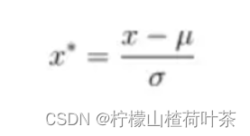
2，5，数据的预处理

# Preprocessing: reshape the image data into rows
X_train = np.reshape(X_train, (X_train.shape[0], -1))
X_val = np.reshape(X_val, (X_val.shape[0], -1))
X_test = np.reshape(X_test, (X_test.shape[0], -1))
X_dev = np.reshape(X_dev, (X_dev.shape[0], -1))

# As a sanity check, print out the shapes of the data
print('Training data shape: ', X_train.shape)
print('Validation data shape: ', X_val.shape)
print('Test data shape: ', X_test.shape)
print('dev data shape: ', X_dev.shape)

还记得在课程的PPT中，我要把图像拉成一个向量后才进行计算的吗？

这里预处理的第一步就是把所有的数据中的图像都展开成一个向量。

比如说这里的X_train展开后的维度是49000行x3072列，说明每张32x32x3的图都被展开成了一个行向量，共49000行。

# Preprocessing: subtract the mean image
# first: compute the image mean based on the training data

mean_image = np.mean(X_train_flatten, axis=0)
#axis=0：按列求均值。
#axis=1：按行求均值。
print("mean_image shape:",mean_image.shape)
print(mean_image[:10]) # print a few of the elements
plt.figure(figsize=(4,4))
plt.imshow(mean_image.reshape((32,32,3)).astype('uint8')) # visualize the mean image
plt.show()

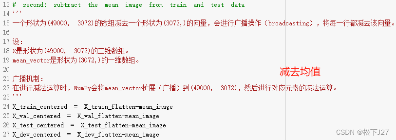
# second: subtract the mean image from train and test data
'''
一个形状为(49000, 3072)的数组减去一个形状为(3072,)的向量，会进行广播操作（broadcasting），将每一行都减去该向量。

设：
X是形状为(49000, 3072)的二维数组。
mean_vector是形状为(3072,)的一维数组。

广播机制：
在进行减法运算时，NumPy会将mean_vector扩展（广播）到(49000, 3072)，然后进行对应元素的减法运算。
'''
X_train_centered = X_train_flatten-mean_image
X_val_centered = X_val_flatten-mean_image
X_test_centered = X_test_flatten-mean_image
X_dev_centered = X_dev_flatten-mean_image

先是求图像的均值，作者采用的是按列求均值的方式，得到的结果是一个3072的向量mean_image。相当于是这个均值向量中的每一个元素都是原来49000张图像在同一位置上所有像素值的均值。

然后，让所有数据集中的图像减去均值mean_image。这里的减法是按行操作的，因为现有二维数据集所保存的数据，每一行就是一幅图。

最后，增加偏置项b，偏置项的每个元素都是一个常数，对应一个类别。以增广矩阵的形式把偏置项，用一个全1的列向量加到所有训练集的最后面。如此一来，在优化权重矩阵W的时候也把偏置项b一起优化了。等权重矩阵W全都优化好以后，之前把矩阵W的最后一列取出来，就得到了优化好的b向量。

X_train_centered = X_train_flatten-mean_image
X_val_centered = X_val_flatten-mean_image
X_test_centered = X_test_flatten-mean_image
X_dev_centered = X_dev_flatten-mean_image

# third: append the bias dimension of ones (i.e. bias trick) so that our SVM
# only has to worry about optimizing a single weight matrix W.
X_train_Preprocessed = np.hstack([X_train_centered, np.ones((X_train.shape[0], 1))])
X_val_Preprocessed = np.hstack([X_val_centered, np.ones((X_val.shape[0], 1))])
X_test_Preprocessed = np.hstack([X_test_centered, np.ones((X_test.shape[0], 1))])
X_dev_Preprocessed = np.hstack([X_dev_centered, np.ones((X_dev.shape[0], 1))])

print("X_train + bias shape:",X_train_Preprocessed.shape)
print("X_val + bias shape:",X_val_Preprocessed.shape)
print("X_test + bias shape:",X_test_Preprocessed.shape)
print("X_dev + bias shape:",X_dev_Preprocessed.shape)

从运行结果上看所有的训练集都在列方向增加了一个维度，从3072变成了3073。

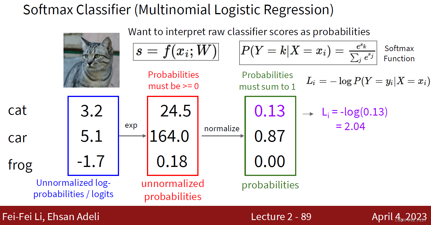
3，assignment coding --- SVM损失函数

前面都是一些准备工作，到这里才真正开始了SVM分类器的部分。主要就是要实现PPT中的下面几个部分：

1，定义一个损失函数去衡量W矩阵的权重是否合理(只不过此处作业指定让我们使用SVM loss)。

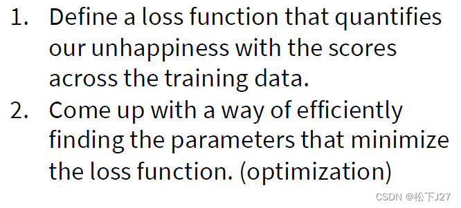
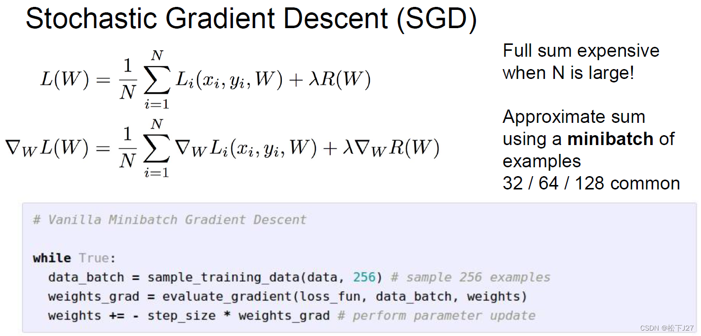
2，选择一种梯度下降法更新W矩阵(作业里指定让我们用SGD)

现在让我们回到官方说明：

他让我们在指定目录下找到“linear_svm.py”文件，然后再在函数“svm_loss_naive”中完成相应代码。（所有这些操作都要在google colab里面完成，系统会自动同步更新代码）

打开指定路径的文件。

在文件中找到对应函数，往下划，就能看到todo list了：

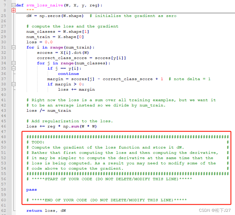
这个函数有四个输入，两个输出。根据主程序的使用范例可知，四个输入分别为权重矩阵W，输入图像X_dev_Preprocessed，输入图像相应的分类标签y_dev，以及正则化系数0.00005。输出是损失函数loss和损失函数相对于权重系数W的偏导数grad。

注意，因为在官方给出的代码中scores的计算公式为score=X[i]*W，且输出为每一类的分数。

再加上对NumPy 库而言，一个形状为 [D,] 的向量X[i]是一个一维向量，而不是严格意义上的行向量或列向量。在 NumPy 中，如果一个形状为 (D,) 的一维向量与一个二维矩阵进行矩阵乘法操作，NumPy 会将这个一维向量自动解释为行向量进行操作，乘法的结果也应该是一个行向量。也就是说X[i]是一个1x3073的矩阵，sroces是一个1xnum_classes的矩阵。因此，W应该是一个3073xnum_classes的矩阵生成对应维度的scores，且默认权重暂时都是随机数。

就本例而言，W=3073x10。

3，1 svm_loss_naive

下面我们看一下官方给出的这个计算损失函数的svm_loss_naive函数究竟在干什么？

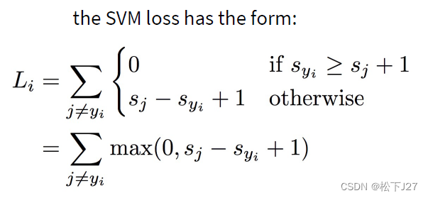
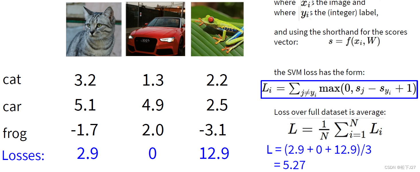
结合课件来看实际上他就实现了两个功能，一个是下面这个方程，这个方程的重点是引入了正则化系数防止过拟合。

另一个是SVM loss function的具体实现，即在score向量中，损失函数的值为其他类的分数减去正确分类的分数后再经过一个非线性操作max之后的和：

结合debug的信息来看能更好的理解官方代码：

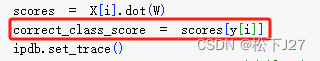
3，1，1 计算第i张图的scores

3，1，2 取出输入图像对应种类的分数，其中，当前图像的种类由y[i]给出。

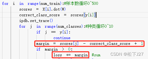
3，1，3 max(0,其他类分数减去正确类分数+1)后求和

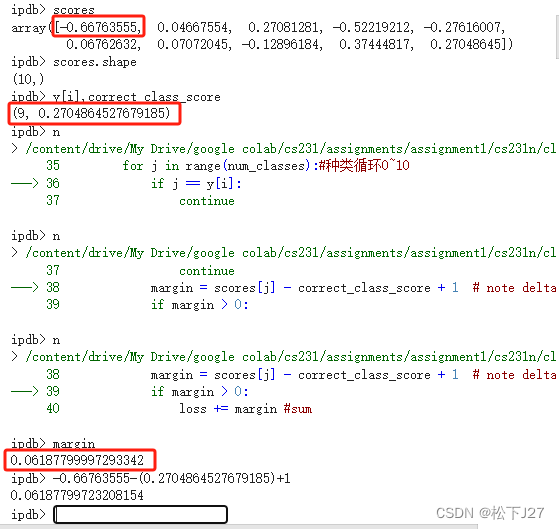
这是第一类的计算结果：

循环十次后得到第一张图像loss的sum。

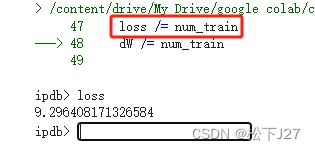
dev子集总共500张图全部计算完毕后，得到总的loss。

最后，求出所有图像loss的均值，return。

Loss函数的值越大表示基于当前权重矩阵W得到的结果越unhappy! 至此，官方说明文档给出的code就全部介绍完了。后面要做的是计算损失函数关于W的偏导数，并使用该偏导数不断地调整W矩阵，直到loss的值小到一定程度后，训练完成，得到我们期望的W。

3，1，4 求梯度dW

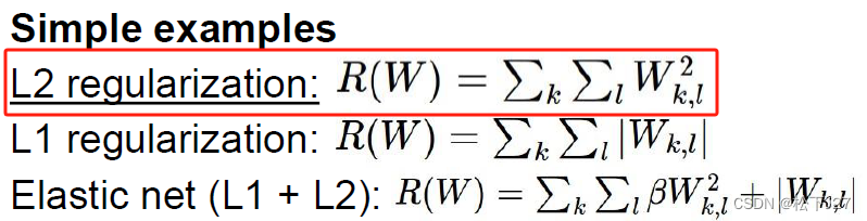
基于官方给出的code和课件可知SVM loss function的计算公式如下：

$L=\frac{1}{N}\sum_{i=1}^{N}\sum_{j=1,j\neq y[i]}^{class}max(0,S[j]-S[y[i]]+\Delta )+Reg$

$where\; \Delta =1,Reg=\lambda R(W)=\lambda W^{2},S_{j}=X_{i}W,class=num \; of\; class,X_{i}=the\: \: i'th\; sample\rightarrow i=1\sim N$

注意，官方给出的code使用的是L2正则化，且偏置项b内化在矩阵W中。

这里，我需要分别求出L关于W的偏导数。在求偏导数之前，我先把上面的公式改写成复合函数的形式：

$L=\frac{1}{N}\sum_{i=1}^{N}L_{i}(f(X_{i},W),y[i])+Reg$

$L_{i}(f(X_{i},W),y[i])=\sum_{j=1,j\neq y[i]}^{class}max(0,S[j]-S[y[i]]+\Delta )$

$S=f(x_{i},W)=X_{i}W+b$

$Reg=\lambda W^{2}$

对于其他分类S[j]而言有：

$\frac{\partial L}{\partial W}=\frac{\partial L}{\partial L_{i}}\cdot \frac{\partial L_{i}}{\partial S[j]}\cdot \frac{\partial S[j]}{\partial W}=1/N\sum_{i=1}^{N}\cdot 1\cdot X_{i}=1/N\sum_{i=1}^{N}X_{i}$

对于已知分类S[y[i]]而言有：

$\frac{\partial L}{\partial W}=\frac{\partial L}{\partial L_{i}}\cdot \frac{\partial L_{i}}{\partial S[y[i]]}\cdot \frac{\partial S[y[i]]}{\partial W}=1/N\sum_{i=1}^{N}\cdot -1\cdot X_{i}=1/N\sum_{i=1}^{N}(-1)X_{i}$

对于正则化函数Reg有：

$\frac{\partial L}{\partial W}=\frac{\partial L}{\partial Reg}\cdot \frac{\partial Reg}{\partial W}= \lambda R(W)=1\cdot 2\lambda W=2\lambda W$

def svm_loss_naive(W, X, y, reg):
    """
    Structured SVM loss function, naive implementation (with loops).

    Inputs have dimension D, there are C classes, and we operate on minibatches
    of N examples.

    Inputs:
    - W: A numpy array of shape (D, C) containing weights.
    - X: A numpy array of shape (N, D) containing a minibatch of data.
    - y: A numpy array of shape (N,) containing training labels; y[i] = c means
      that X[i] has label c, where 0 <= c < C.
    - reg: (float) regularization strength

    Returns a tuple of:
    - loss as single float
    - gradient with respect to weights W; an array of same shape as W
    """
    dW = np.zeros(W.shape)  # initialize the gradient as zero

    # compute the loss and the gradient
    num_classes = W.shape[1]
    num_train = X.shape[0]
    loss = 0.0
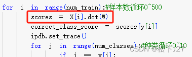
    for i in range(num_train):#样本数循环0~500
        scores = X[i].dot(W)
        correct_class_score = scores[y[i]]
        #ipdb.set_trace()
        for j in range(num_classes):#种类循环0~10
            if j == y[i]:
                continue
            margin = scores[j] - correct_class_score + 1  # note delta = 1
            if margin > 0:
                loss += margin #sum
                #########################################################
                #         START OF CHANGE          #
                #########################################################
                dW[:, j] += X[i]    # For incorrect class
                dW[:, y[i]] -= X[i]   # For correct class
                #########################################################
                #          END OF CHANGE          #
                #########################################################

    # Right now the loss is a sum over all training examples, but we want it
    # to be an average instead so we divide by num_train.
    ipdb.set_trace()
    loss /= num_train

    # Add regularization to the loss.
    loss += reg * np.sum(W * W)


    #############################################################################
    # TODO:                                                                     #
    # Compute the gradient of the loss function and store it dW.                #
    # Rather that first computing the loss and then computing the derivative,   #
    # it may be simpler to compute the derivative at the same time that the     #
    # loss is being computed. As a result you may need to modify some of the    #
    # code above to compute the gradient.                                       #
    #############################################################################
    # *****START OF YOUR CODE (DO NOT DELETE/MODIFY THIS LINE)*****
    
    # scale gradient ovr the number of samples
    dW /= num_train

    # append partial derivative of regularization term
    dW += 2 * reg * W
    
    # *****END OF YOUR CODE (DO NOT DELETE/MODIFY THIS LINE)*****

    return loss, dW

矩阵dW是一个维度为3073x10的矩阵。第张0图像的计算结果dW如下所示：

dW的第一列等于X[0].

dW的第二列等于X[0].

...

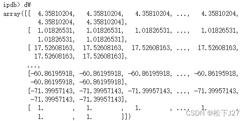
从code中可以看出，除了第y[i]列外dW的每一列都等于输入图像X[0]，只有第y[i]列的值等于输入图像X[0]的负值的累加，总共累加9次（共分10类）。

在j不等于y[i]的地方，总共有多少处大于0的margin就要累加多少次！

完成500张图像的循环后，最终得到的loss和dW如下。

3，1，5 验证梯度

这一步的作用是用直接根据导数的定义用数值计算的方法求得的梯度来验证上面自己写的SVM LOSS NAIVE函数中用代数法求出的梯度是否准确，两者之间的误差应该非常小才对。

# Once you've implemented the gradient, recompute it with the code below
# and gradient check it with the function we provided for you

# Compute the loss and its gradient at W.
loss, grad = svm_loss_naive(W, X_dev_Preprocessed, y_dev, 0.0)

# Numerically compute the gradient along several randomly chosen dimensions, and
# compare them with your analytically computed gradient. The numbers should match
# almost exactly along all dimensions.
from cs231n.gradient_check import grad_check_sparse
print("check gradient with Reg=0")
f = lambda w: svm_loss_naive(w, X_dev_Preprocessed, y_dev, 0.0)[0]
grad_numerical = grad_check_sparse(f, W, grad)

# do the gradient check once again with regularization turned on
# you didn't forget the regularization gradient did you?
loss, grad = svm_loss_naive(W, X_dev_Preprocessed, y_dev, 5e1)
print("check gradient with Reg=50")
f = lambda w: svm_loss_naive(w, X_dev_Preprocessed, y_dev, 5e1)[0]
grad_numerical = grad_check_sparse(f, W, grad)

此外这段代码分别验证了带正则项与不带正则项的计算。

3，1，6 用矩阵运算加速SVM LOSS FUNCTION的计算

对于单张图像而言，当margin>0时，dW其他类的列等于X[i]，而正确类的列等于-(num of margin>0)*X[i]。开发集总共有500张图，每新增一张图都要累加到前面的结果上。

矩阵dW是一个维度为3073x10的矩阵,每一列表示的是500张图在第j类上的综合贡献。第0张图对于第一列(即第一类)的贡献应该是X[0]乘以这张图在第j类上的权重（若为正确类，则权重为-(num of margin>0)。若为其他类则权重为1）。第1张图对于第一列(即第一类)的贡献应该是X[1]乘以这张图在第j类上的权重。依此类推，得到500张图片对第一列的贡献应该是矩阵X(X矩阵共500行，每行是一张图的3072个像素)第一行与500个不同权重的线性组合。

又因为是行操作因此应该是前乘行的方式。相当于是X前乘以一个1x500的行向量作为结果的第一行（需转置后变成第一列），和X前乘以一个1x500的行向量作为结果的第二列（需转置后变成第二行），依此类推共10行，最后转置得到我们想要的dW。

再依此类推，把第一行与500个不同权重的线性组合，第二行与500个不同权重的线性组合，。。。第十行与500个不同权重的线性组合的计算合并到一起得到权重矩阵X_w与输入矩阵X的乘积。

def svm_loss_vectorized(W, X, y, reg):
    """
    Structured SVM loss function, vectorized implementation.

    Inputs and outputs are the same as svm_loss_naive.
    """
    loss = 0.0
    dW = np.zeros(W.shape)  # initialize the gradient as zero

    #############################################################################
    # TODO:                                                                     #
    # Implement a vectorized version of the structured SVM loss, storing the    #
    # result in loss.                                                           #
    #############################################################################
    # *****START OF YOUR CODE (DO NOT DELETE/MODIFY THIS LINE)*****

    # number of samples
    N=len(y)
    # 计算所有样本的分数,每行10个score共500行。
    scores=X@W
    print(scores.shape)
    # 逐行选出每个样本的正确类别的分数
    correct_class_scores = scores[range(N),y]
    print(correct_class_scores.shape)
    # 拓展为对应维度的二维矩阵
    correct_class_scores=correct_class_scores[:, np.newaxis]
    print(correct_class_scores.shape)
    # 计算所有样本的SVM loss,结果是一个500x10的矩阵。
    # 每行的结果是一张图10分类的分数相对正确类分数的计算结果，共计500行。
    margins = np.maximum(0, scores - correct_class_scores + 1)
    print(margins.shape)
    margins[range(N), y] = 0  # 将正确类别的损失置0，不参与统计
    loss = np.sum(margins) / N  # 求所有图像的平均损失
    loss += reg * np.sum(W * W)  # 添加正则化项

    # *****END OF YOUR CODE (DO NOT DELETE/MODIFY THIS LINE)*****

    #############################################################################
    # TODO:                                                                     #
    # Implement a vectorized version of the gradient for the structured SVM     #
    # loss, storing the result in dW.                                           #
    #                                                                           #
    # Hint: Instead of computing the gradient from scratch, it may be easier    #
    # to reuse some of the intermediate values that you used to compute the     #
    # loss.                                                                     #
    #############################################################################
    # *****START OF YOUR CODE (DO NOT DELETE/MODIFY THIS LINE)*****

    # 计算梯度
    ipdb.set_trace()
    X_w = np.zeros(margins.shape)
    X_w[margins > 0] = 1 # mask中margin中大于0的地方为1，其余为0.(整体处理)
    row_sum = np.sum(X_w, axis=1)# 统计每张图margin中大于0的num.(行处理)
    X_w[np.arange(N), y] = -row_sum# 找到每一行正确类的位置，并赋值为负的row_sum.(行处理)
    dW = X.T@X_w / N #（X_w'*X)'=X'*X_w

    # 添加正则化项的梯度
    dW += 2 * reg * W

    # *****END OF YOUR CODE (DO NOT DELETE/MODIFY THIS LINE)*****

    return loss, dW

以下是debug模式下X_w矩阵的构建过程：

完成好向量化的SVM loss就可以用官方给的代码去验证计算结果和计算时间了。实际上向量化的SVM loss与之前的naive SVM loss的唯一区别就是前者使用了矩阵运算大大的加快了计算速度。

这是计算loss和统计计算时长的函数

# Next implement the function svm_loss_vectorized; for now only compute the loss;
# we will implement the gradient in a moment.
tic = time.time()
loss_naive, _ = svm_loss_naive(W, X_dev_Preprocessed, y_dev, 0.000005)
toc = time.time()
print('Naive loss: %e computed in %fs' % (loss_naive, toc - tic))

from cs231n.classifiers.linear_svm import svm_loss_vectorized
tic = time.time()
loss_vectorized, _ = svm_loss_vectorized(W, X_dev_Preprocessed, y_dev, 0.000005)
toc = time.time()
print('Vectorized loss: %e computed in %fs' % (loss_vectorized, toc - tic))

# The losses should match but your vectorized implementation should be much faster.
print('difference: %f' % (loss_naive - loss_vectorized))

实验结果，二者的loss一样，但矩阵运算快了0.087s。

这是计算grad和统计计算时长的函数

# Complete the implementation of svm_loss_vectorized, and compute the gradient
# of the loss function in a vectorized way.

# The naive implementation and the vectorized implementation should match, but
# the vectorized version should still be much faster.
tic = time.time()
_, grad_naive = svm_loss_naive(W, X_dev_Preprocessed, y_dev, 0.000005)
toc = time.time()
print('Naive loss and gradient: computed in %fs' % (toc - tic))

tic = time.time()
_, grad_vectorized = svm_loss_vectorized(W, X_dev_Preprocessed, y_dev, 0.000005)
toc = time.time()
print('Vectorized loss and gradient: computed in %fs' % (toc - tic))

# The loss is a single number, so it is easy to compare the values computed
# by the two implementations. The gradient on the other hand is a matrix, so
# we use the Frobenius norm to compare them.
difference = np.linalg.norm(grad_naive - grad_vectorized, ord='fro')
print('difference: %f' % difference)

同样梯度相同，计算速度快了不少。

3，1，7 用梯度下降法更新W

官方给出的用于测试的code

# In the file linear_classifier.py, implement SGD in the function
# LinearClassifier.train() and then run it with the code below.
from cs231n.classifiers import LinearSVM
svm = LinearSVM()
tic = time.time()
loss_hist = svm.train(X_train_Preprocessed, y_train, learning_rate=1e-7, reg=2.5e4,
                      num_iters=1500, verbose=True)
toc = time.time()
print('That took %fs' % (toc - tic))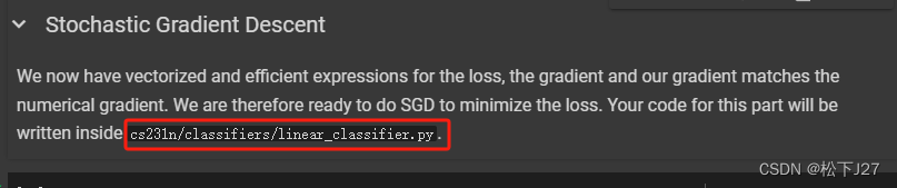

需要自己手写的部分

from __future__ import print_function

from builtins import range
from builtins import object
import numpy as np
from ..classifiers.linear_svm import *
from ..classifiers.softmax import *
from past.builtins import xrange


class LinearClassifier(object):
    def __init__(self):
        self.W = None

    def train(
        self,
        X,
        y,
        learning_rate=1e-3,
        reg=1e-5,
        num_iters=100,
        batch_size=200,
        verbose=False,
    ):
        """
        Train this linear classifier using stochastic gradient descent.

        Inputs:
        - X: A numpy array of shape (N, D) containing training data; there are N
          training samples each of dimension D.
        - y: A numpy array of shape (N,) containing training labels; y[i] = c
          means that X[i] has label 0 <= c < C for C classes.
        - learning_rate: (float) learning rate for optimization.
        - reg: (float) regularization strength.
        - num_iters: (integer) number of steps to take when optimizing
        - batch_size: (integer) number of training examples to use at each step.
        - verbose: (boolean) If true, print progress during optimization.

        Outputs:
        A list containing the value of the loss function at each training iteration.
        """
        num_train, dim = X.shape
        num_classes = (
            np.max(y) + 1
        )  # assume y takes values 0...K-1 where K is number of classes
        if self.W is None:
            # lazily initialize W
            self.W = 0.001 * np.random.randn(dim, num_classes)

        # Run stochastic gradient descent to optimize W
        loss_history = []
        for it in range(num_iters):
            X_batch = None
            y_batch = None

            #########################################################################
            # TODO:                                                                 #
            # Sample batch_size elements from the training data and their           #
            # corresponding labels to use in this round of gradient descent.        #
            # Store the data in X_batch and their corresponding labels in           #
            # y_batch; after sampling X_batch should have shape (batch_size, dim)   #
            # and y_batch should have shape (batch_size,)                           #
            #                                                                       #
            # Hint: Use np.random.choice to generate indices. Sampling with         #
            # replacement is faster than sampling without replacement.              #
            #########################################################################
            # *****START OF YOUR CODE (DO NOT DELETE/MODIFY THIS LINE)*****

            # 在num_train当中随机采样batch_size个样本
            indices = np.random.choice(num_train, batch_size, replace=True)
            X_batch = X[indices]
            y_batch = y[indices]

            # *****END OF YOUR CODE (DO NOT DELETE/MODIFY THIS LINE)*****

            # evaluate loss and gradient
            loss, grad = self.loss(X_batch, y_batch, reg)
            loss_history.append(loss)

            # perform parameter update
            #########################################################################
            # TODO:                                                                 #
            # Update the weights using the gradient and the learning rate.          #
            #########################################################################
            # *****START OF YOUR CODE (DO NOT DELETE/MODIFY THIS LINE)*****

            self.W -= learning_rate * grad

            # *****END OF YOUR CODE (DO NOT DELETE/MODIFY THIS LINE)*****

            if verbose and it % 100 == 0:
                print("iteration %d / %d: loss %f" % (it, num_iters, loss))

        return loss_history

    def predict(self, X):
        """
        Use the trained weights of this linear classifier to predict labels for
        data points.

        Inputs:
        - X: A numpy array of shape (N, D) containing training data; there are N
          training samples each of dimension D.

        Returns:
        - y_pred: Predicted labels for the data in X. y_pred is a 1-dimensional
          array of length N, and each element is an integer giving the predicted
          class.
        """
        y_pred = np.zeros(X.shape[0])
        ###########################################################################
        # TODO:                                                                   #
        # Implement this method. Store the predicted labels in y_pred.            #
        ###########################################################################
        # *****START OF YOUR CODE (DO NOT DELETE/MODIFY THIS LINE)*****

        #ipdb.set_trace()
        y_pred = np.argmax(X@(self.W), axis=1)

        # *****END OF YOUR CODE (DO NOT DELETE/MODIFY THIS LINE)*****
        return y_pred

    def loss(self, X_batch, y_batch, reg):
        """
        Compute the loss function and its derivative.
        Subclasses will override this.

        Inputs:
        - X_batch: A numpy array of shape (N, D) containing a minibatch of N
          data points; each point has dimension D.
        - y_batch: A numpy array of shape (N,) containing labels for the minibatch.
        - reg: (float) regularization strength.

        Returns: A tuple containing:
        - loss as a single float
        - gradient with respect to self.W; an array of the same shape as W
        """
        pass


class LinearSVM(LinearClassifier):
    """ A subclass that uses the Multiclass SVM loss function """

    def loss(self, X_batch, y_batch, reg):
        return svm_loss_vectorized(self.W, X_batch, y_batch, reg)


class Softmax(LinearClassifier):
    """ A subclass that uses the Softmax + Cross-entropy loss function """

    def loss(self, X_batch, y_batch, reg):
        return softmax_loss_vectorized(self.W, X_batch, y_batch, reg)

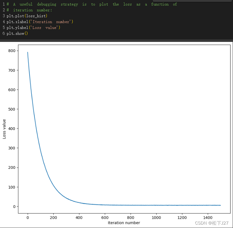
相应的计算结果如下所示：

3，1，8 使用训练集和验证集来评估模型的性能

# Write the LinearSVM.predict function and evaluate the performance on both the
# training and validation set
y_train_pred = svm.predict(X_train_Preprocessed)
print('training accuracy: %f' % (np.mean(y_train == y_train_pred), ))
y_val_pred = svm.predict(X_val_Preprocessed)
print('validation accuracy: %f' % (np.mean(y_val == y_val_pred), ))

要点：

结果：

解释：

训练集准确率和验证集准确率是否相同反映了模型的泛化性能。

过拟合（Overfitting）：
- 当模型在训练集上表现非常好，达到高准确率，但在验证集上表现较差时，通常意味着模型过拟合了训练数据。过拟合的模型学习到了训练数据中的噪声和特定模式，而不是数据的普遍特征。
- 过拟合的表现是训练集准确率高，而验证集准确率低。
欠拟合（Underfitting）：
- 如果模型在训练集上和验证集上都表现不佳，准确率都很低，这说明模型欠拟合。欠拟合的模型没有捕捉到数据中的重要模式和特征。
- 欠拟合的表现是训练集和验证集准确率都低。

3，1，9 使用不同的学习率和正则化系数去训练模型，找到最优超参数

# Use the validation set to tune hyperparameters (regularization strength and
# learning rate). You should experiment with different ranges for the learning
# rates and regularization strengths; if you are careful you should be able to
# get a classification accuracy of about 0.39 (> 0.385) on the validation set.

# Note: you may see runtime/overflow warnings during hyper-parameter search.
# This may be caused by extreme values, and is not a bug.

# results is dictionary mapping tuples of the form
# (learning_rate, regularization_strength) to tuples of the form
# (training_accuracy, validation_accuracy). The accuracy is simply the fraction
# of data points that are correctly classified.
results = {}
best_val = -1   # The highest validation accuracy that we have seen so far.
best_svm = None # The LinearSVM object that achieved the highest validation rate.

################################################################################
# TODO:                                                                        #
# Write code that chooses the best hyperparameters by tuning on the validation #
# set. For each combination of hyperparameters, train a linear SVM on the      #
# training set, compute its accuracy on the training and validation sets, and  #
# store these numbers in the results dictionary. In addition, store the best   #
# validation accuracy in best_val and the LinearSVM object that achieves this  #
# accuracy in best_svm.                                                        #
#                                                                              #
# Hint: You should use a small value for num_iters as you develop your         #
# validation code so that the SVMs don't take much time to train; once you are #
# confident that your validation code works, you should rerun the validation   #
# code with a larger value for num_iters.                                      #
################################################################################

# Provided as a reference. You may or may not want to change these hyperparameters
learning_rates = [1e-9, 2e-8, 1e-7]
regularization_strengths = [2.5e4, 5e4, 6e6]

# *****START OF YOUR CODE (DO NOT DELETE/MODIFY THIS LINE)*****

# 创建一个 LinearSVM 对象
svm = LinearSVM()

# 循环遍历 learning_rates 和 regularization_strengths
for lr in learning_rates:
    for reg in regularization_strengths:

        # 调整模型的超参数和评估模型的性能，以避免过拟合
        loss_history = svm.train(X_train_Preprocessed, y_train, learning_rate=lr, reg=reg,
                                 num_iters=1500, verbose=False)

        # 训练后，计算准确率
        y_train_pred = svm.predict(X_train_Preprocessed)
        train_accuracy = np.mean(y_train == y_train_pred)

        y_val_pred = svm.predict(X_val_Preprocessed)
        val_accuracy = np.mean(y_val == y_val_pred)

        # 将准确率存储在 results 字典中
        results[(lr, reg)] = (train_accuracy, val_accuracy)

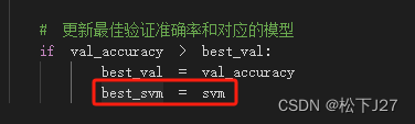
        # 更新最佳验证准确率和对应的模型
        if val_accuracy > best_val:
            best_val = val_accuracy
            best_svm = svm

# *****END OF YOUR CODE (DO NOT DELETE/MODIFY THIS LINE)*****

# Print out results.
for lr, reg in sorted(results):
    train_accuracy, val_accuracy = results[(lr, reg)]
    print('lr %e reg %e train accuracy: %f val accuracy: %f' % (
                lr, reg, train_accuracy, val_accuracy))

print('best validation accuracy achieved during cross-validation: %f' % best_val)

实验结果：

先是尝试了4个不同数量级的学习率和4个正则化系数

得到如下结果：

可见当学习率为e-7次方数量级时，准确率最高。而当学习率为e-3次方数量级时，准确率最低。此外，当学习率为e-7次方时，正则化系数在e+2次方达到最大，并随着e次方的增加而越来越小。因此，可以把学习率控制在e-7附近和正则化系数在e+2附近。

重新调整学习率和Reg后：

得到新的实验结果如下：

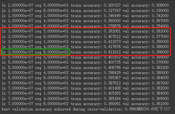
可见，学习率在3e-7时的准确率最高，其中又以Reg=8e+2时达到所有组合中的最大值。最终把最优模型返回给best_svm

3，1，10 在测试集上测试最优模型

# Evaluate the best svm on test set
y_test_pred = best_svm.predict(X_test_Preprocessed)
test_accuracy = np.mean(y_test == y_test_pred)
print('linear SVM on raw pixels final test set accuracy: %f' % test_accuracy)

3，1，11 训练好的权重矩阵W的可视化

# Visualize the learned weights for each class.
# Depending on your choice of learning rate and regularization strength, these may
# or may not be nice to look at.
w = best_svm.W[:-1,:] # strip out the bias
w = w.reshape(32, 32, 3, 10)
w_min, w_max = np.min(w), np.max(w)
classes = ['plane', 'car', 'bird', 'cat', 'deer', 'dog', 'frog', 'horse', 'ship', 'truck']
for i in range(10):
    plt.subplot(2, 5, i + 1)

    # Rescale the weights to be between 0 and 255
    wimg = 255.0 * (w[:, :, :, i].squeeze() - w_min) / (w_max - w_min)
    plt.imshow(wimg.astype('uint8'))
    plt.axis('off')
    plt.title(classes[i])