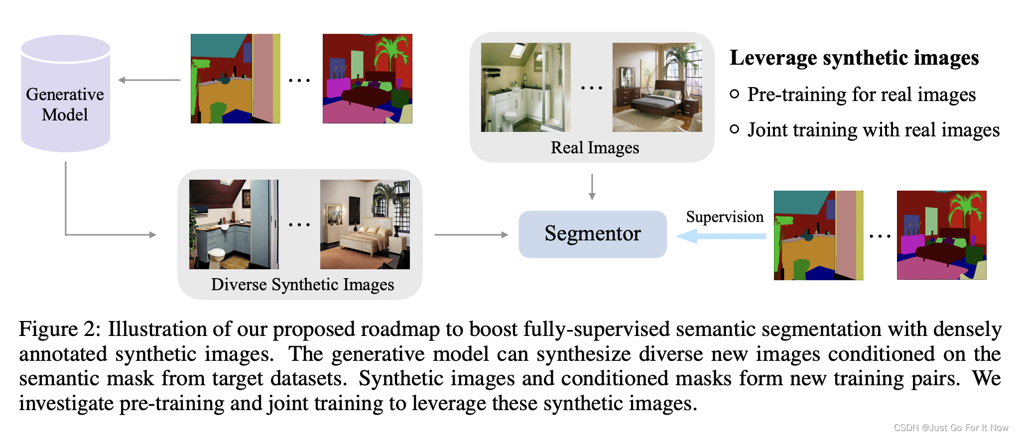
Real-data WRF | setup and run and experiment - 酸梨子-专注技术分享

前言

Parent Model = 用于初始化和边界条件的网格数据

GFS/FNL、NAM、RAP/HRRR、重新分析（NARR、CFSR、NNRP、ERA-interim、ERA5 等）、其他 WRF 运行

WPS = WRF 预处理系统（由 geogrid、ungrib 和 metgrid 程序组成）

WRF 模拟几乎总是使用 GRIB1/2 格式的等压水平上的模型数据集或 NetCDF 格式的 WRF 输出进行初始化

WRF 输出几乎总是 NetCDF

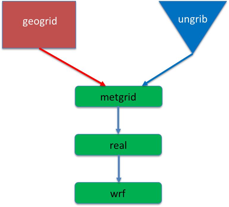
模式运行流程图：

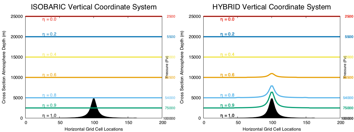
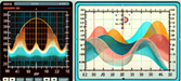
其中，初始场数据几乎总是以等压水平(isobaric levels )提供（如左图所示）。
Metgrid 将等压数据插值到 WRF 水平网格上。 Real 将 metgrid 数据插值到 WRF 垂直网格上，这是一个混合地形跟随坐标（如右图所示）。 WRFV4相对于之前的版本进一步改进了这个坐标。

WRF整体包括WPS前处理和WRF后处理，在进行WPS之前，需要链接数据类型，以及驱动模式的初始场和边界层数据。

链接运行数据的类型变量，以ERA5数据为例：

ln -sf ungrib/Variable_Tables/Vtable.ECMWF Vtable

链接你下载的初始场和边界数据，根据你数据放置的文件夹进行链接,这里以下载的ERA5数据为例：

./link_grib.csh ./ERA5_data/*

WPS

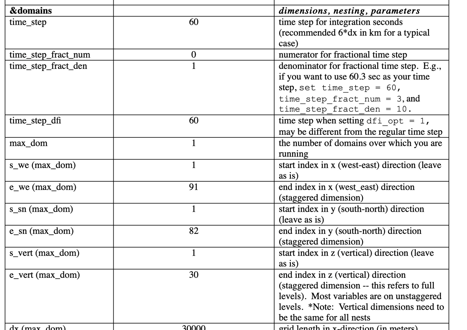
一般在namelist.wps 中设置模拟区域的分辨率、区域大小、模拟时间等，namelist.input中的分辨率、区域大小、模拟时间等变量应与namelist.wps 中的设置一致。

依次运行以下模拟步骤

1、Geogrid (geogrid.exe)

设置域（和嵌套，如果适用），在此环节中：创建 geo_em.d01.nc文件，仅在模拟区域更改时重做；

在运行./geogrid.exe 命令之前，可以使用ncl util/plotgrids_new.ncl 进行测试，得到模拟区域：

2、Ungrib (ungrib.exe)

解压 GRIB1 和 GRIB2 父模型数据，几乎总是在等压(isobaric levels)水平上, 需要正确的变量表（“Vtable”）转换器，在此环节中：创建许多名为 FILE:* 的文件

3、Metgrid (metgrid.exe)

将解压的初始模型数据插值到 WRF 模型（水平）网格,在此环节中：创建许多名为 met_em.d01.* 的文件

WRF

主要边界的信息在namelist.input中（用于real.exe、wrf.exe）

4、Real (real.exe)

将 metgrid 输出从初始数据的的垂直坐标插值到 WRF 的垂直坐标，在地形跟随的 WRF 垂直网格上创建初始和边界条件文件。在本环节中：创建 wrfinput_d01 和 wrfbdy_d01文件

5、WRF (wrf.exe)

编译为 em_real，从 real 读取初始和边界条件文件。在此环节中：输出文件名类似为 wrfout_d01_2023-01-22_12:00:00 的数据

下面具体展开进行介绍

准备工作

namelist.wps（用于 geogrid.exe、ungrib.exe、metgrid.exe）

&share
 wrf_core = 'ARW',
 max_dom = 1,
 start_date ='2023-01-22_12:00:00', '2023-01-22_12:00:00'
 end_date =  '2023-01-24_00:00:00', '2023-01-24_00:00:00'
 interval_seconds = 10800,
 io_form_geogrid = 2,
 opt_output_from_geogrid_path = './',
 debug_level = 0
/

注意点：

一个模拟区域 (max_dom = 1)，因此 start_date 的第二列和end_date并不重要
Interval_Seconds 是初始场数据的时间分辨率（以秒为单位）
（对于 GFS，我们有 3 小时的数据，因此 10800 秒）
（NAM 为每小时 36 小时，此后每小时 3 小时）
/ 和下一个 & 之间的任何内容都会被忽略
对于geogrid步骤，此时只有本节中的 max_dom 设置很重要

&geogrid
 parent_id         =   1,   1,   2,
 parent_grid_ratio =   1,   3,   3,
 i_parent_start    =   1, 82, 100,
 j_parent_start    =   1, 82,  36,
 s_we              =   1,   1,   1,
 e_we              = 54, 214, 772,
 s_sn              =  1,   1,   1,
 e_sn              = 48, 196, 610,
 geog_data_res     ='default', 'default', 'default',
 dx        =  36000.,
 dy        =  36000.,
 map_proj  = 'lambert',
 ref_lat   =  43.,
 ref_lon   = -74,
 truelat1  =  43.,
 truelat2  =  43.,
 stand_lon = -74,
 geog_data_path = '/network/rit/lab/atm419lab/GEOG4.0/',
 opt_geogrid_tbl_path = 'geogrid/'
/

注意：：

同样，在这种情况下，只有第一列重要,因为 max_dom = 1
我们的单一域为 54 x 48 和 36 公里（分辨率）网格间距
我们使用“默认”土地利用数据库……MODIS 21 类别（其他可用还有USGS 24-category land use categories）
兰伯特投影是中纬度地区中等大小区域的标准投影。
对于高纬度地区使用极地赤极坐标，对于热带地区使用墨卡托坐标。

地图

在 namelist.wps 中指定 Δx（和 Δy）
地图因子 m 决定实际网格间距：

因此，当 m > 1.0 时，实际网格间距小于指定的 Δx。这会给你的时间步带来压力。
当 m < 1.0 时，您的分辨率比您想象的要低。尽可能接近 1.0。

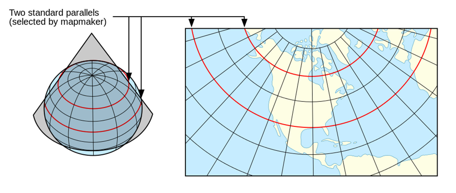
兰伯特等形投影(Lambert conformal projection )（来自维基百科）

形状和精度在某种程度上取决于“真实纬度”（标准纬线）

 ref_lat   =  43.,
 ref_lon   = -74,
 truelat1  =  43.,
 truelat2  =  43.,
 stand_lon = -74,

在true latitude，不存在地图扭曲；
即地图因子为 1.0。默认为 30 和 60°。对于相对较小的域，真实纬度可以相等（如此处）并设置为中心纬度。

地图系数=（水平网格尺寸）/（实际距离），所以当因子 > 1 时，你的实际网格大小 < Δx, Δy

这里可以给出一个对比测试的例子：

区域1

 ref_lat   =  38.5,
 ref_lon   = -121.5,
 truelat1  =  38.5,
 truelat2  =  38.5,
 stand_lon = -121.5,

区域2

 ref_lat   =  38.5,
 ref_lon   = -121.5,
 truelat1  =  38.5,
 truelat2  =  38.5,
 stand_lon = -151.5,

Example of ref_lon ≠ stand_lon

&share
 wrf_core = 'ARW',
 max_dom = 1,
 start_date ='2023-01-22_12:00:00', '2016-03-13_00:00:00'
 end_date =  '2023-01-24_00:00:00', '2016-03-15_00:00:00'
 interval_seconds = 10800,
 io_form_geogrid = 2,
 opt_output_from_geogrid_path = './',
 debug_level = 0
/

&ungrib
 out_format = 'WPS',
 prefix     = 'FILE',
/

&metgrid
 fg_name         = 'FILE',
 io_form_metgrid = 2,
/

注意点：

执行ungrib.exe 将网格解压到一组由前缀命名的文件（此处为“FILE:…”）
程序按时间间隔查找,开始日期和结束日期之间的文件指定为间隔秒
metgrid.exe 是下一个，它将查找名为FILE:…的文件

绘制 ungrib.exe 创建的中间格式文件

使用以下命令：

ncl plotfmt.ncl 'filename="FILE:2023-01-22_12"'

metgrid

在此步骤中，我们将中间格式文件中的数据放置到 WRF 水平网格上，创建名为 met_em* 的文件
可以使用 ncview（较差）或 IDV（较好）或 Python 查看文件

对任何 met_em* 文件使用 ncdump 来获取垂直高度数和土壤高度数

ncdump -h met_em.d01.2023-01-22_12:00:00.nc | more

netcdf met_em.d01.2023-01-22_12\:00\:00 {
dimensions:
	Time = UNLIMITED ; // (1 currently)
	DateStrLen = 19 ;
	west_east = 53 ;
	south_north = 47 ;
	num_metgrid_levels = 34 ;
	num_st_layers = 4 ;
	num_sm_layers = 4 ;
	south_north_stag = 48 ;
	west_east_stag = 54 ;
	z-dimension0003 = 3 ;
	z-dimension0132 = 132 ;
	z-dimension0012 = 12 ;
	z-dimension0016 = 16 ;
	z-dimension0021 = 21 ;

此初始场数据，包含：

34 vertical atmospheric levels
4 soil temperature and soil
moisture layers (st and sm)

运行真实数据 WRF（real.exe 和 wrf.exe）通常会占用大量资源，无法从命令行使用 srun 执行。
作为替代方案，我们将它们作为批处理作业在集群上运行。 SETUP.TAR提供了两个文件：submit_real和submit_wrf。

两者目前都配置为在单个节点上请求 8 个 cpu,此时无需编辑这些脚本（如果您愿意，更改您的作业名称除外）

#!/bin/bash
# Job name:
#SBATCH --job-name=atm419
#SBATCH -n 8
#SBATCH -N 1
#SBATCH --mem=131072
#SBATCH -o sbatch.out
#SBATCH -e sbatch.err.out

st_tm="$(date +%s)"

echo "running real"
srun -N 1 -n 8 --mpi=pmix -o real.srun.out ./real.exe

其中，#SBATCH -n 8,#SBATCH -N 1需要与-N 1 -n 8保持一致。

然后，提交作业即可，提交作业后，当作业从队列中消失时，使用tail命令检查 rsl.out.0000 文件的尾部。

如： tail -f rsl.out.0000

d01 2023-01-24_00:00:00 real_em：SUCCESS COMPLETE REAL_EM INIT

real.exe 的结果：创建文件 wrfbdy_d01 和 wrfinput_d01。如果这些文件已经存在，它们将被覆盖。

同样的，运行./wrf.exe 会得到的结果：创建 wrfout_d01_2023-01-22_12:00:00 文件
如果该文件已经存在，则会被覆盖。

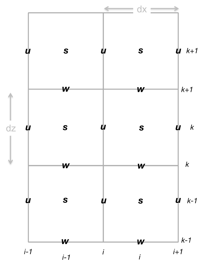
WRF网格

WRF uses a horizontally
 and vertically staggered
 grid


u = east-west velocity
w = vertical velocity
s = scalar field

One extra W point in vertical
One extra U point west-east
One extra V point north-south

u(i,k), w(i,k) and s(i,k) do not represent same physical locations (in wrfout files)!
[Some postprocessing tools de-stagger the grid for you]

horizontally and vertically staggered grid

后处理脚本

绘制地形terrain

import numpy as np
import matplotlib.pyplot as plt
from matplotlib.cm import get_cmap
from matplotlib.colors import from_levels_and_colors
import cartopy.crs as ccrs
import cartopy.feature as cf
from netCDF4 import Dataset
from wrf import (getvar, to_np, get_cartopy, latlon_coords, vertcross, ll_to_xy,
                 cartopy_xlim, cartopy_ylim, interpline, CoordPair, destagger, 
                 interplevel)

# set filename and its location
location = "/nfs/atm419lab/TESTING/SNOW/” # EDIT THIS WITH LOCATION OF YOUR FILE
file = ”wrfinput_d01"

# combine location and filename
ncfile = Dataset(location + file)

# extract variables from wrf output
hgt = getvar(ncfile,"HGT")               # terrain height
latwrf = getvar(ncfile,"XLAT")           # latitude
lonwrf = getvar(ncfile,"XLONG")          # longitude
plt.figure(figsize=(9, 12))

lat_0 = 38                     # ref_lat from namelist.wps
lon_0 = -100                   # ref_lon from namelist.wps
standard_parallels = (38.,38.) # truelat1, truelat2 from namelist.wps

proj=ccrs.LambertConformal(central_latitude=lat_0, central_longitude=lon_0, 
                           standard_parallels=standard_parallels, globe=None)
ax = plt.axes(projection=proj)

ax.add_feature(cf.COASTLINE.with_scale('10m'))
ax.add_feature(cf.BORDERS.with_scale('10m'))
ax.add_feature(cf.LAKES,alpha=0.5) # alpha sets transparency level
ax.add_feature(cf.RIVERS)
ax.add_feature(cf.STATES.with_scale('10m'),linestyle='dotted')

norm = plt.Normalize(0, 4000)
cm = ax.contourf(lonwrf,latwrf,hgt,norm=norm,cmap=plt.cm.terrain,
                 transform=ccrs.PlateCarree())

# colorbar
plt.colorbar(cm, orientation="vertical",fraction=0.02, pad=0.04)
plt.show()

namelist.input 介绍

namelist.input

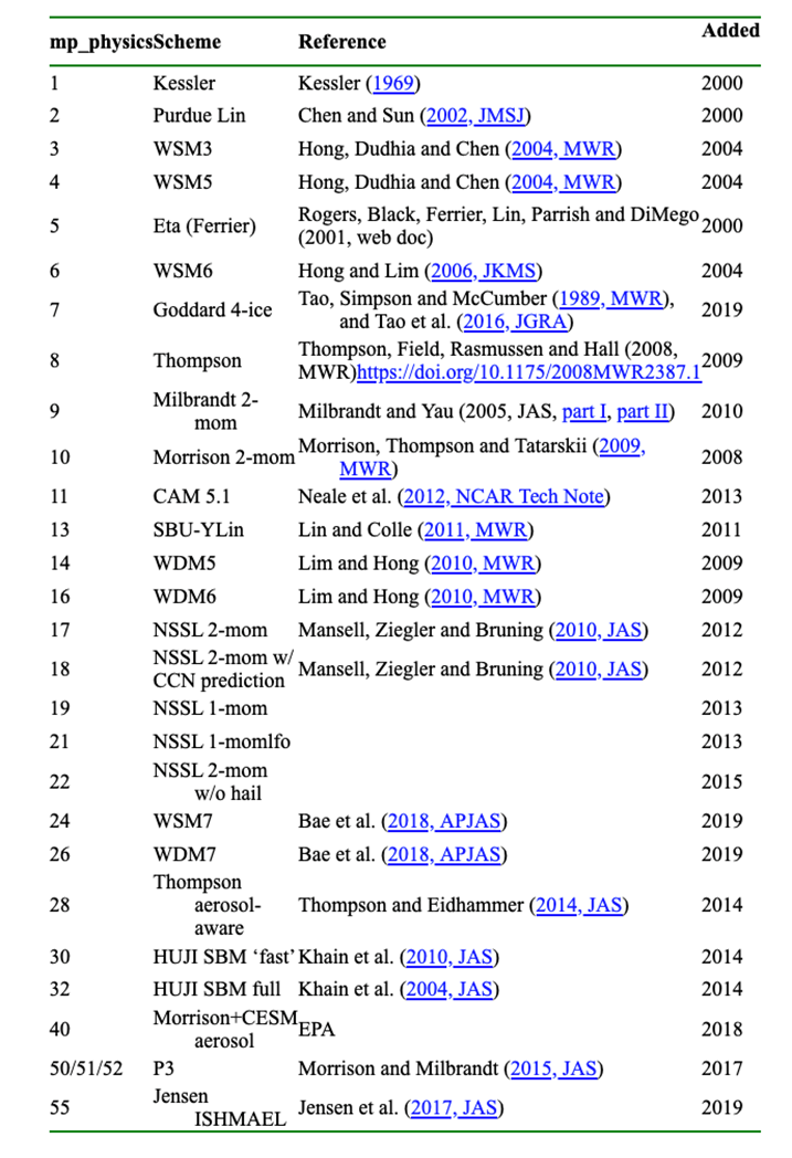
云微物理方案：

mp_physics scheme

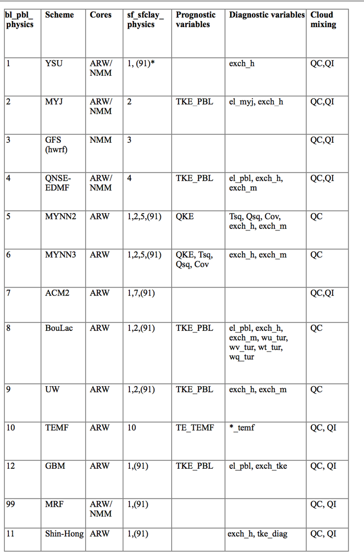
边界层方案

Some available PBL schemes:

  YSU: pbl = 1, sfclay = 1
  MYJ: pbl = 2, sfclay = 2
  MYNN: pbl = 5, sfclay = 1, 2, or 5
  ACM2: pbl = 7, sfclay = 7

Some land surface models:

 Noah: surface = 2, soil = 4
 NoahMP: surface = 4, soil = 4
 TD: surface = 1, soil = 5
 RUC: surface = 3, soil = 6 or 9
 PX: surface = 7, soil = 2
 CLM: surface = 5, 10

pbl =  bl_pbl_physics
sfclay = sf_sfclay_physics
surface = sf_surface_physics
soil = num_soil_layers

PBL schemes

以下是主要的参考资料：

WRFV4 users guide (PDF available):
http://www2.mmm.ucar.edu/wrf/users/docs/user_guide_v4/contents.html

Technical description of WRFV4 (PDF):
https://www2.mmm.ucar.edu/wrf/users/docs/technote/v4_technote.pdf

NetCDF operators (NCO) home page: https://nco.sourceforge.net/

封面来源：
https://lair.utah.edu/page/project/biomass/WRF_data/index.html