- 🍨 本文为🔗365天深度学习训练营 中的学习记录博客
- 🍖 原作者:K同学啊 | 接辅导、项目定制
数据链接
提取码:o3ix
目录
0. 总结
数据导入部分:本次数据导入没有使用torchvision自带的数据集,需要将原始数据进行处理包括数据导入,数据类型转换,划定训练集测试集后,再使用torch.utils.data中的DataLoader()加载数据
模型构建部分:有两个部分一个初始化部分(init())列出了网络结构的所有层,比如卷积层池化层等。第二个部分是前向传播部分,定义了数据在各层的处理过程。
设置超参数:在这之前需要定义损失函数,学习率,以及根据学习率定义优化器(例如SGD随机梯度下降),用来在训练中更新参数,最小化损失函数。
定义训练函数:函数的传入的参数有四个,分别是设置好的DataLoader(),定义好的模型,损失函数,优化器。函数内部初始化损失准确率为0,接着开始循环,使用DataLoader()获取一个批次的数据,对这个批次的数据带入模型得到预测值,然后使用损失函数计算得到损失值。接下来就是进行反向传播以及使用优化器优化参数,梯度清零放在反向传播之前或者是使用优化器优化之后都是可以的。将 optimizer.zero_grad() 放在了每个批次处理的开始,这是最标准和常见的做法。这样可以确保每次迭代处理一个新批次时,梯度是从零开始累加的。准确率是通过累计预测正确的数量得到的,处理每个批次的数据后都要不断累加正确的个数,最终的准确率是由预测正确的数量除以所有样本得数量得到的。损失值也是类似每次循环都累计损失值,最终的损失值是总的损失值除以训练批次得到的
定义测试函数:函数传入的参数相比训练函数少了优化器,只需传入设置好的DataLoader(),定义好的模型,损失函数。此外除了处理批次数据时无需再设置梯度清零、返向传播以及优化器优化参数,其余部分均和训练函数保持一致。
训练过程:定义训练次数,有几次就使用整个数据集进行几次训练,初始化四个空list分别存储每次训练及测试的准确率及损失。使用model.train()开启训练模式,调用训练函数得到准确率及损失。使用model.eval()将模型设置为评估模式,调用测试函数得到准确率及损失。接着就是将得到的训练及测试的准确率及损失存储到相应list中并合并打印出来,得到每一次整体训练后的准确率及损失。
模型的保存,调取及使用。在PyTorch中,通常使用 torch.save(model.state_dict(), ‘model.pth’) 保存模型的参数,使用 model.load_state_dict(torch.load(‘model.pth’)) 加载参数。
需要改进优化的地方:再保证整体流程没有问题的情况下,继续细化细节研究,比如一些函数的原理及作用,如何提升训练集准确率等问题。
1. 数据导入部分
import torch
import torch.nn as nn
import torchvision
from torchvision import transforms,datasets

import os,PIL,pathlib,random

device = torch.device("cuda" if torch.cuda.is_available() else "cpu")
device
device(type='cuda')
# 数据导入部分
data_dir = './data/weather_recognize/weather_photos/'
data_dir = pathlib.Path(data_dir)

data_paths = list(data_dir.glob('*')) # 获取左右子文件名称
# classNames = [str(path).split("\\")[3] for path in data_paths] # ['cloudy', 'rain', 'shine', 'sunrise']
classNames = [path.parts[-1] for path in data_paths]
classNames
['cloudy', 'rain', 'shine', 'sunrise']
# 数据展示
import matplotlib.pyplot as plt
from PIL import Image # Pillow 是一个图像处理库,可以用来打开、操作和保存许多不同格式的图像文件。

# 指定图像文件夹路径
image_folder = './data/weather_recognize/weather_photos/cloudy/'

# 获取文件夹中的所有图像文件
image_files = [f for f in os.listdir(image_folder) if f.endswith((".jpg",".png",".jpeg"))]

# 创建Matplotlib图像

fig,axes = plt.subplots(3,8,figsize=(16,6))

# 使用列表推导式加载和显示图像
for ax,img_file in zip(axes.flat,image_files):
    img_path = os.path.join(image_folder,img_file)
    img = Image.open(img_path)
    ax.imshow(img)
    ax.axis('off')

# 显示图像
plt.tight_layout()
plt.show()

# 数据格式转换
total_datadir = './data/weather_recognize/weather_photos/'

# 关于transforms.Compose的更多介绍可以参考:https://blog.csdn.net/qq_38251616/article/details/124878863
train_transforms = torchvision.transforms.Compose([
    transforms.Resize([224,224]), # 输入图片resize成统一尺寸
    transforms.ToTensor(),        # 将PIL Image或numpy.ndarray转换为tensor,并归一化到[0,1]之间
    transforms.Normalize(         # 其中 mean=[0.485,0.456,0.406]与std=[0.229,0.224,0.225] 从数据集中随机抽样计算得到的。
        mean = [0.485,0.456,0.406],
        std = [0.229,0.224,0.225]
    )
])

total_data = torchvision.datasets.ImageFolder(total_datadir,transform=train_transforms)
total_data
Dataset ImageFolder
    Number of datapoints: 1125
    Root location: ./data/weather_recognize/weather_photos/
    StandardTransform
Transform: Compose(
               Resize(size=[224, 224], interpolation=bilinear, max_size=None, antialias=warn)
               ToTensor()
               Normalize(mean=[0.485, 0.456, 0.406], std=[0.229, 0.224, 0.225])
           )
# 划分数据集
train_size = int(0.8 * len(total_data))
test_size = len(total_data) - train_size
train_dataset,test_dataset = torch.utils.data.random_split(total_data, [train_size, test_size])
train_dataset,test_dataset
(<torch.utils.data.dataset.Subset at 0x21120a68460>,
 <torch.utils.data.dataset.Subset at 0x2115a4ec7f0>)
# 使用dataloader加载数据,并设置好基本的batch_size
batch_size = 32

train_dl = torch.utils.data.DataLoader(
    train_dataset,
    batch_size = batch_size,
    shuffle = True,
    num_workers = 1 # 用于数据加载的子进程数量。通常,将其设置为大于 0 的值可以加快数据加载速度,特别是当数据集很大时。默认值为 0,表示在主进程中加载数据。
)
test_dl = torch.utils.data.DataLoader(
    test_dataset,
    batch_size = batch_size,
    shuffle = True,
    num_workers = 1
)
# 查看数据
for X,y in test_dl:
    print("Shape of X[N,C,H,W]: ",X.shape)
    print("Shape of y: ",y.shape,y.dtype)
    break
Shape of X[N,C,H,W]:  torch.Size([32, 3, 224, 224])
Shape of y:  torch.Size([32]) torch.int64
数据导入部分代码详解:
a. 数据读取部分
●第一步:使用pathlib.Path()函数将字符串类型的文件夹路径转换为pathlib.Path对象。
●第二步:使用glob()方法获取data_dir路径下的所有文件路径,并以列表形式存储在data_paths中。
●第三步:
通过split()函数对data_paths中的每个文件路径执行分割操作,获得各个文件所属的类别名称,并存储在classeNames中.
或直接使用pathlib的.parts方法
●第四步:打印classeNames列表,显示每个文件所属的类别名称。
a.1 提问:关于这段代码,我想知道为什么split函数中用以分割的是"\“符号而不是”/"
回答:
在这段代码中,split("\\")[3] 被用来从文件路径中提取特定的部分。这里使用反斜杠(\)而不是正斜杠(/)作为分隔符,可能是因为这段代码原本是为在 Windows 系统上运行而编写的。在 Windows 文件系统中,路径通常使用反斜杠 \ 作为分隔符。例如,一个典型的 Windows 文件路径可能看起来像这样:C:\Users\UserName\Documents\File.txt。
但是,值得注意的是,Python 的 pathlib 库是跨平台的,并会自动处理不同操作系统中的路径分隔符差异。当使用 pathlib 处理文件路径时,通常不需要手动指定分隔符。事实上,使用 pathlib 的方法(如 .parts 或 .name)通常更为安全和可靠,因为它们可以适应不同的操作系统。
例如,如果目的是获取路径中的某个特定部分(如这里的类名),可以使用 pathlib 提供的属性而不是手动分割字符串。如果 data_paths 中的路径是类似于 ./data/weather_recognize/weather_photos/ClassName/FileName.jpg 的格式,那么可以这样获取类名:
classNames = [path.parts[-2] for path in data_paths]
这样就无需关心是使用 \ 还是 / 作为分隔符,代码会更加健壮,适用于不同的操作系统。
a.2 提问2:可以为我介绍一下pathlib的.parts和.name方法吗
回答2:
当然可以。pathlib 是 Python 的一个标准库,用于面向对象地处理文件系统路径。它提供了多种方法来操作和提取路径信息,其中 .parts 和 .name 是两个非常实用的属性。
.parts
.parts返回一个表示路径各部分的元组。- 它将整个路径分解为其组成部分,每个部分由路径中的一个目录或文件名表示。
- 在不同的操作系统中,路径的分隔符可能不同(例如,在 Windows 中是
\,在 Unix 和 macOS 中是/),但.parts会自动处理这些差异。 - 示例:
- 假设有一个路径
Path("/usr/bin/python3"),.parts将返回('/', 'usr', 'bin', 'python3')。 - 在 Windows 系统上,对于
Path("C:\\Users\\UserName\\Documents\\File.txt"),.parts将返回('C:\\', 'Users', 'UserName', 'Documents', 'File.txt')。
- 假设有一个路径
.name
.name返回路径中最后一部分的名称。- 对于文件路径,它返回文件名;对于目录路径,它返回目录名。
- 它不包括路径中的任何父目录部分。
- 示例:
- 对于路径
Path("/usr/bin/python3"),.name将返回python3。 - 对于路径
Path("C:\\Users\\UserName\\Documents\\File.txt"),.name将返回File.txt。
- 对于路径
使用 pathlib 的这些属性可以让路径处理更加直观和安全,尤其是在处理跨平台的路径问题时。
b. 用列表推导式加载和显示图像代码的逐行解释:
for ax, img_file in zip(axes.flat, image_files):- 这是一个 for 循环,使用
zip函数来同时遍历axes.flat(所有子图对象的扁平化列表)和image_files(图像文件名列表)。ax是当前子图的引用,img_file是当前要处理的图像文件名。
- 这是一个 for 循环,使用
img_path = os.path.join(image_folder, img_file)- 使用
os.path.join构建完整的图像文件路径。这个函数能正确处理不同操作系统中的路径分隔符。
- 使用
img = Image.open(img_path)- 使用 Pillow 的
Image.open方法打开图像文件。
- 使用 Pillow 的
ax.imshow(img)- 在当前的子图(
ax)上显示图像img。
- 在当前的子图(
ax.axis('off')- 关闭当前子图的坐标轴,这样图像就不会显示任何坐标轴标签或刻度。
plt.tight_layout()- 调整子图的布局,使得图像之间没有太大的间隙,并确保子图的标题和轴标签不会重叠。
plt.show()- 显示最终的图像。这通常会弹出一个窗口显示所有的图像。
2. 模型构建部分
3, 224, 224(输入数据)
-> 12, 220, 220(经过卷积层1)
-> 12, 216, 216(经过卷积层2)-> 12, 108, 108(经过池化层1)
-> 24, 104, 104(经过卷积层3)
-> 24, 100, 100(经过卷积层4)-> 24, 50, 50(经过池化层2)
-> 60000 -> num_classes(4)
# 模型构建
import torch.nn.functional as F

class Network_bn(nn.Module):
    def __init__(self):
        super(Network_bn,self).__init__()
        self.conv1 = nn.Conv2d(in_channels = 3,out_channels = 12,kernel_size = 5,stride = 1,padding = 0)
        self.bn1 = nn.BatchNorm2d(12)
        self.conv2 = nn.Conv2d(in_channels = 12,out_channels = 12,kernel_size = 5,stride = 1,padding = 0)
        self.bn2 = nn.BatchNorm2d(12)
        self.pool = nn.MaxPool2d(2,2)
        self.conv3 = nn.Conv2d(in_channels = 12,out_channels = 24,kernel_size = 5,stride = 1,padding = 0)
        self.bn3 = nn.BatchNorm2d(24)
        self.conv4 = nn.Conv2d(in_channels = 24,out_channels = 24,kernel_size = 5,stride = 1,padding = 0)
        self.bn4 = nn.BatchNorm2d(24)
        self.dropout = nn.Dropout(p=0.5)     # 尝试在全连接层之前加入dropout,减少过拟合
        self.fc1 = nn.Linear(24*50*50,len(classNames)) # 尝试加入多个全连接层提升模型性能
        # self.fc2 = nn.Linear(30000,15000)             # 尝试加入多个全连接层提升模型性能
        # self.fc3 = nn.Linear(30000,len(classNames))   # 尝试加入多个全连接层提升模型性能

    def forward(self,x):
        x = F.relu(self.bn1(self.conv1(x)))
        x = F.relu(self.bn2(self.conv2(x)))
        x = self.pool(x)
        x = F.relu(self.bn3(self.conv3(x)))
        x = F.relu(self.bn4(self.conv4(x)))
        x = self.pool(x)
        x = x.view(-1,24*50*50)
        # x = self.dropout(x)
        x = F.relu(self.fc1(x)) # 在全连接层之间添加激活函数
        # x = self.dropout(x)     # 尝试将dropout层放置在两个全连接层之间
        # x = F.relu(self.fc2(x)) # 在全连接层之间添加激活函数
        # x = F.relu(self.fc3(x)) # 在全连接层之间添加激活函数
        return x

print("Using {} device".format(device))

model = Network_bn().to(device)
model
Using cuda device


Network_bn(
  (conv1): Conv2d(3, 12, kernel_size=(5, 5), stride=(1, 1))
  (bn1): BatchNorm2d(12, eps=1e-05, momentum=0.1, affine=True, track_running_stats=True)
  (conv2): Conv2d(12, 12, kernel_size=(5, 5), stride=(1, 1))
  (bn2): BatchNorm2d(12, eps=1e-05, momentum=0.1, affine=True, track_running_stats=True)
  (pool): MaxPool2d(kernel_size=2, stride=2, padding=0, dilation=1, ceil_mode=False)
  (conv3): Conv2d(12, 24, kernel_size=(5, 5), stride=(1, 1))
  (bn3): BatchNorm2d(24, eps=1e-05, momentum=0.1, affine=True, track_running_stats=True)
  (conv4): Conv2d(24, 24, kernel_size=(5, 5), stride=(1, 1))
  (bn4): BatchNorm2d(24, eps=1e-05, momentum=0.1, affine=True, track_running_stats=True)
  (dropout): Dropout(p=0.5, inplace=False)
  (fc1): Linear(in_features=60000, out_features=4, bias=True)
)
计算公式:
卷积维度计算公式:
高度方向:$ H_{out} = \frac{\left(H_{in} - Kernel_size + 2\times padding\right)}{stride} + 1 $
宽度方向:$ W_{out} = \frac{\left(W_{in} - Kernel_size + 2\times padding\right)}{stride} + 1 $
卷积层通道数变化:数据通道数为卷积层该卷积层定义的输出通道数,例如:self.conv1 = nn.Conv2d(3,64,kernel_size = 3)。在这个例子中,输出的通道数为64,这意味着卷积层使用了64个不同的卷积核,每个核都在输入数据上独立进行卷积运算,产生一个新的通道。需要注意,卷积操作不是在单独的通道上进行的,而是跨所有输入通道(本例中为3个通道)进行的,每个卷积核提供一个新的输出通道。
池化层计算公式:
高度方向: H o u t = ( H i n + 2 × p a d d i n g H − d i l a t i o n H × ( k e r n e l _ s i z e H − 1 ) − 1 s t r i d e H + 1 ) H_{out} = \left(\frac{H_{in} + 2 \times padding_H - dilation_H \times (kernel\_size_H - 1) - 1}{stride_H} + 1 \right) Hout=(strideHHin+2×paddingH−dilationH×(kernel_sizeH−1)−1+1)
宽度方向: W o u t = ( W i n + 2 × p a d d i n g W − d i l a t i o n W × ( k e r n e l _ s i z e W − 1 ) − 1 s t r i d e W + 1 ) W_{out} = \left( \frac{W_{in} + 2 \times padding_W - dilation_W \times (kernel\_size_W - 1) - 1}{stride_W} + 1 \right) Wout=(strideWWin+2×paddingW−dilationW×(kernel_sizeW−1)−1+1)
其中:
- H i n H_{in} Hin 和 W i n W_{in} Win 是输入的高度和宽度。
- p a d d i n g H padding_H paddingH 和 p a d d i n g W padding_W paddingW 是在高度和宽度方向上的填充量。
- k e r n e l _ s i z e H kernel\_size_H kernel_sizeH 和 k e r n e l _ s i z e W kernel\_size_W kernel_sizeW 是卷积核或池化核在高度和宽度方向上的大小。
- s t r i d e H stride_H strideH 和 s t r i d e W stride_W strideW 是在高度和宽度方向上的步长。
- d i l a t i o n H dilation_H dilationH 和 d i l a t i o n W dilation_W dilationW 是在高度和宽度方向上的膨胀系数。
请注意,这里的膨胀系数 $dilation \times (kernel_size - 1) $实际上表示核在膨胀后覆盖的区域大小。例如,一个 $3 \times 3 $ 的核,如果膨胀系数为2,则实际上它覆盖的区域大小为$ 5 \times 5 $(原始核大小加上膨胀引入的间隔)。
计算流程:
输入数据:( 3 ∗ 224 ∗ 224 3*224*224 3∗224∗224)
conv1计算:卷积核数12,输出的通道也为12。-> ( 12 ∗ 220 ∗ 220 ) (12*220*220) (12∗220∗220)
输出维度 = ( 224 − 5 + 2 × 0 ) 1 + 1 = 220 \text{输出维度} = \frac{\left(224 - 5 + 2 \times 0\right)}{1} + 1 = 220 输出维度=1(224−5+2×0)+1=220
conv2计算:-> ( 12 ∗ 216 ∗ 216 ) (12*216*216) (12∗216∗216)
输出维度 = ( 220 − 5 + 2 × 0 ) 1 + 1 = 216 \text{输出维度} = \frac{\left(220 - 5 + 2 \times 0\right)}{1} + 1 = 216 输出维度=1(220−5+2×0)+1=216
pool1计算:通道数不变,步长为2-> ( 12 ∗ 108 ∗ 108 ) (12*108*108) (12∗108∗108)
输出维度 = ( 216 + 2 × 0 − 1 × ( 2 − 1 ) − 1 2 + 1 ) = 107 + 1 = 108 \text{输出维度} = \left(\frac{216 + 2 \times 0 - 1 \times \left(2 - 1\right) - 1}{2} + 1 \right) = 107 +1 = 108 输出维度=(2216+2×0−1×(2−1)−1+1)=107+1=108
conv3计算:-> ( 24 ∗ 104 ∗ 104 ) (24*104*104) (24∗104∗104)
输出维度 = ( 108 − 5 + 2 × 0 ) 1 + 1 = 104 \text{输出维度} = \frac{\left(108 - 5 + 2 \times 0\right)}{1} + 1 = 104 输出维度=1(108−5+2×0)+1=104
conv4计算:-> ( 24 ∗ 100 ∗ 100 ) (24*100*100) (24∗100∗100)
输出维度 = ( 104 − 5 + 2 × 0 ) 1 + 1 = 100 \text{输出维度} = \frac{\left(104 - 5 + 2 \times 0\right)}{1} + 1 = 100 输出维度=1(104−5+2×0)+1=100
pool2计算:-> ( 24 ∗ 50 ∗ 50 ) (24*50*50) (24∗50∗50)
输出维度 = ( 100 + 2 × 0 − 1 × ( 2 − 1 ) − 1 2 + 1 ) = 49 + 1 = 50 \text{输出维度} = \left(\frac{100 + 2 \times 0 - 1 \times \left(2 - 1\right) - 1}{2} + 1 \right) = 49 +1 = 50 输出维度=(2100+2×0−1×(2−1)−1+1)=49+1=50
flatten层:-> 60000 60000 60000
n u m _ c l a s s e s ( 4 ) num\_classes(4) num_classes(4)
3. 设置超参数
loss_fn = nn.CrossEntropyLoss() # 创建损失函数
learn_rate = 1e-4 # 学习率
opt = torch.optim.SGD(model.parameters(),lr=learn_rate)
# opt = torch.optim.Adam(model.parameters(),lr=learn_rate)
4. 训练函数
# 训练循环
def train(dataloader,model,loss_fn,optimizer):
    size = len(dataloader.dataset)
    num_batches = len(dataloader)

    train_loss,train_acc = 0,0

    for X,y in dataloader:
        X,y = X.to(device),y.to(device)

        # 计算预测值
        pred = model(X)
        loss = loss_fn(pred,y)

        # 反向传播
        optimizer.zero_grad()
        loss.backward()
        optimizer.step()

        # 记录acc与loss
        train_acc += (pred.argmax(1)==y).type(torch.float).sum().item()
        train_loss += loss.item()

    train_loss /= num_batches
    train_acc /= size

    return train_acc,train_loss
5. 测试函数
# 测试函数
def test(dataloader,model,loss_fn):
    size = len(dataloader.dataset)
    num_batches = len(dataloader)

    test_acc,test_loss = 0,0
    # 当不进行梯度训练时,停止梯度更新,节省计算内存消耗
    with torch.no_grad():
        for X,y in dataloader:
            X,y = X.to(device),y.to(device)

            # 计算预测值
            pred = model(X)
            loss = loss_fn(pred,y)

            test_acc += (pred.argmax(1) == y).type(torch.float).sum().item()
            test_loss += loss.item()

    test_acc /= size
    test_loss /= num_batches

    return test_acc,test_loss
6. 训练过程
epochs = 20
train_loss = []
train_acc = []
test_loss = []
test_acc = []
for epoch in range(epochs):
model.train()
epoch_train_acc,epoch_train_loss = train(train_dl,model,loss_fn,opt)
model.eval()
epoch_test_acc,epoch_test_loss = test(test_dl,model,loss_fn)
train_acc.append(epoch_train_acc)
train_loss.append(epoch_train_loss)
test_acc.append(epoch_test_acc)
test_loss.append(epoch_test_loss)
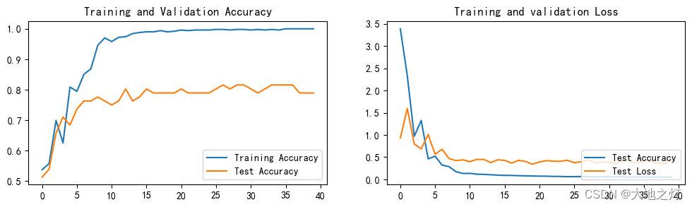
template = ('Epoch:{:2d},Train_acc:{:.1f}%,Train_loss:{:.3f},Test_acc:{:.1f}%,Test_loss:{:.3f}')
print(template.format(epoch+1,epoch_train_acc*100,epoch_train_loss,epoch_test_acc*100,epoch_test_loss))
print('Done!')
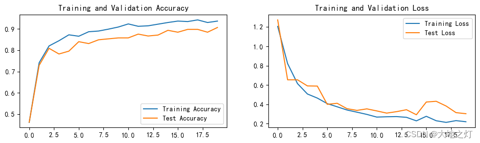
Epoch: 1,Train_acc:46.1%,Train_loss:1.207,Test_acc:46.2%,Test_loss:1.274
Epoch: 2,Train_acc:74.1%,Train_loss:0.822,Test_acc:72.9%,Test_loss:0.654
Epoch: 3,Train_acc:82.0%,Train_loss:0.614,Test_acc:80.9%,Test_loss:0.654
Epoch: 4,Train_acc:84.4%,Train_loss:0.507,Test_acc:78.2%,Test_loss:0.591
Epoch: 5,Train_acc:87.2%,Train_loss:0.465,Test_acc:79.6%,Test_loss:0.589
Epoch: 6,Train_acc:86.6%,Train_loss:0.408,Test_acc:84.0%,Test_loss:0.400
Epoch: 7,Train_acc:88.7%,Train_loss:0.375,Test_acc:83.1%,Test_loss:0.411
Epoch: 8,Train_acc:89.0%,Train_loss:0.341,Test_acc:84.9%,Test_loss:0.355
Epoch: 9,Train_acc:89.9%,Train_loss:0.319,Test_acc:85.3%,Test_loss:0.337
Epoch:10,Train_acc:90.9%,Train_loss:0.296,Test_acc:85.8%,Test_loss:0.353
Epoch:11,Train_acc:92.3%,Train_loss:0.268,Test_acc:85.8%,Test_loss:0.332
Epoch:12,Train_acc:91.2%,Train_loss:0.271,Test_acc:87.6%,Test_loss:0.309
Epoch:13,Train_acc:91.4%,Train_loss:0.273,Test_acc:86.7%,Test_loss:0.324
Epoch:14,Train_acc:92.2%,Train_loss:0.265,Test_acc:87.1%,Test_loss:0.344
Epoch:15,Train_acc:93.0%,Train_loss:0.229,Test_acc:89.3%,Test_loss:0.292
Epoch:16,Train_acc:93.7%,Train_loss:0.276,Test_acc:88.4%,Test_loss:0.424
Epoch:17,Train_acc:93.4%,Train_loss:0.230,Test_acc:89.8%,Test_loss:0.431
Epoch:18,Train_acc:94.2%,Train_loss:0.213,Test_acc:89.8%,Test_loss:0.382
Epoch:19,Train_acc:93.0%,Train_loss:0.231,Test_acc:88.4%,Test_loss:0.314
Epoch:20,Train_acc:93.7%,Train_loss:0.220,Test_acc:90.7%,Test_loss:0.303
Done!
# 结果可视化
import matplotlib.pyplot as plt
#隐藏警告
import warnings
warnings.filterwarnings("ignore")               #忽略警告信息
plt.rcParams['font.sans-serif']    = ['SimHei'] # 用来正常显示中文标签
plt.rcParams['axes.unicode_minus'] = False      # 用来正常显示负号
plt.rcParams['figure.dpi']         = 100        #分辨率

epochs_range = range(epochs)

plt.figure(figsize=(12, 3))
plt.subplot(1, 2, 1)

plt.plot(epochs_range, train_acc, label='Training Accuracy')
plt.plot(epochs_range, test_acc, label='Test Accuracy')
plt.legend(loc='lower right')
plt.title('Training and Validation Accuracy')

plt.subplot(1, 2, 2)
plt.plot(epochs_range, train_loss, label='Training Loss')
plt.plot(epochs_range, test_loss, label='Test Loss')
plt.legend(loc='upper right')
plt.title('Training and Validation Loss')
plt.show()
7. 模型的保存及调用模型进行预测
# 1.保存模型

# torch.save(model, 'model.pth') # 保存整个模型
torch.save(model.state_dict(), 'model_state_dict.pth') # 仅保存状态字典

# 2. 加载模型 or 新建模型加载状态字典

# model2 = torch.load('model.pth')
# model2 = model2.to(device) # 理论上在哪里保存模型,加载模型也会优先在哪里,但是指定一下确保不会出错

model2 = Network_bn().to(device) # 重新定义模型
model2.load_state_dict(torch.load('model_state_dict.pth')) # 加载状态字典到模型

# 3.图片预处理
from PIL import Image
import torchvision.transforms as transforms

# 输入图片预处理
def preprocess_image(image_path):
    image = Image.open(image_path)
    transform = transforms.Compose([
        transforms.Resize((224, 224)),  # 假设使用的是224x224的输入
        transforms.ToTensor(),
        transforms.Normalize(mean=[0.485, 0.456, 0.406], std=[0.229, 0.224, 0.225]),
    ])
    image = transform(image).unsqueeze(0)  # 增加一个批次维度
    return image

# 4.预测函数(指定路径)
def predict(image_path, model):
    model.eval()  # 将模型设置为评估模式
    with torch.no_grad():  # 关闭梯度计算
        image = preprocess_image(image_path)
        image = image.to(device)  # 确保图片在正确的设备上
        outputs = model(image)
        _, predicted = torch.max(outputs, 1)  # 获取最可能的预测类别
        return predicted.item()

# 5.预测并输出结果
image_path = "./data/weather_recognize/weather_photos/shine/shine22.jpg"  # 替换为你的图片路径
prediction = predict(image_path, model)
class_names = ["cloudy", "rain", "shine", "sunrise"]  # Replace with your class labels
predicted_label = class_names[prediction]
print("Predicted class:", predicted_label)
Predicted class: shine
# 选取dataloader中的一个图像进行判断
import numpy as np
# 选取图像
imgs,labels = next(iter(train_dl))
image,label = imgs[0],labels[0]

# 选取指定图像并展示
# 调整维度为 [224, 224, 3]
image_to_show = image.numpy().transpose((1, 2, 0))

# 归一化
mean = np.array([0.485, 0.456, 0.406])
std = np.array([0.229, 0.224, 0.225])
image_to_show = std * image_to_show + mean
image_to_show = np.clip(image_to_show, 0, 1)

# 显示图像
plt.imshow(image_to_show)
plt.show()

# 将图像转移到模型所在的设备上(如果使用GPU)
image = image.to(device)

# 预测
with torch.no_grad():
    output = model(image.unsqueeze(0))  # 添加批次维度

# 输出预测结果
_, predicted = torch.max(output, 1)
class_names = ["cloudy", "rain", "shine", "sunrise"]  # Replace with your class labels
predicted_label = class_names[predicted]
print(f"Predicted: {predicted.item()}, Actual: {label.item()}")
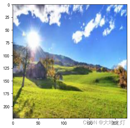
Predicted: 2, Actual: 2


![Cocos2dx-lua ScrollView[三]高级篇](https://img-blog.csdnimg.cn/direct/6b3c230be38d46f688e1c12f7c07b39a.gif)