| info | |
|---|---|
| paper | https://arxiv.org/abs/2401.17270 |
| code | https://github.com/AILab-CVC/YOLO-World |
| org | 腾讯 |
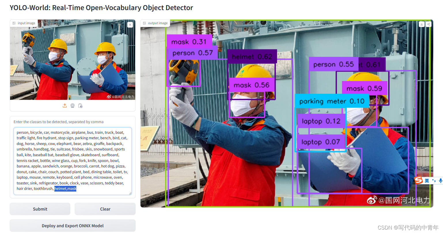
| demo | https://huggingface.co/spaces/stevengrove/YOLO-World |
| 个人博客位置 | http://www.myhz0606.com/article/yolo_world |
1 Motivation
这篇文章从计算效率的角度解决开集目标检测问题(open-vocabulary object detection,OVD)。


2 Method
经典的目标检测的instance annotation是bounding box和类别对 Ω = { B i , c i } i = 1 N \Omega = \{ B_i, c_i\}^{N}_{i=1} Ω={ Bi,ci}i=1N。对于OVD来说,此时的注释变为 Ω = { B i , t i } i = 1 N \Omega = \{ B_i, t_i\}^{N}_{i=1} Ω={ Bi,ti}i=1N,此处的 t t t可以是类别名、名词短语、目标描述等。此外YOLO-Word还可以根据传入的图片和text,输出预测的box及相关的object embedding。
2.1 模型架构

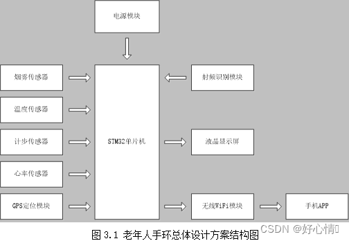
模型架构由3个部分组成
YOLO backbone,用于提取多尺度的图片特征text encoder,用于提取名词短语的特征。流程如下:给定一段text,首先会提取里面的名词,随后将提取的每个名词短语输入CLIP中得到向量。可以知道text encoder的输出 W W W ∈ R C × D \in \mathbb{R} ^{C \times D} ∈RC×D, C C C是名词短语的数量, D D D是embedding的维度Vision-Language PAN。用于预测bounding box和object embedding。其架构如下图所示,核心组件有两个,分别为Text-guided CSPLayer及Image-Pooling Attention。下面对其进行简单介绍
Text-guided CSPLayer
该层的目的是为了用文本向量来强化图片特征。具体计算公式如下
X l ′ = X l ⋅ δ ( max j ∈ { 1.. C } ( X l W j ⊤ ) ) ⊤ (1) X _ { l } ^ { \prime } = X _ { l } \cdot \delta ( \max _ { j \in \{ 1 . . C \} } ( X _ { l } W _ { j } ^ { \top } ) ) ^ { \top } \tag{1} Xl′=Xl⋅δ(j∈{ 1..C}max(XlWj⊤))⊤(1)
式中: X l ∈ R H × W × D ( l ∈ { 3 , 4 , 5 } ) X _ { l } \, \in \, \mathbb { R } ^ { \, H \times W \times D } \, ( l \, \in \, \{ 3 , 4 , 5 \} ) Xl∈RH×W×D(l∈{ 3,4,5}) 为多尺度的图片特征。 W j W_j Wj为名词 j j j的text embedding。 δ \delta δ为sigmoid函数。

**Image-Pooling Attention**
该层的目的是为了用图片特征来强化文本向量。具体做法为:将多尺度图片特征通过max pooling,每个尺度经过max-pooling后的size ∈ R 3 × 3 × D \in \mathbb{R} ^ {3 \times 3 \times D} ∈R3×3×D即9个patch token,因为有3个尺度,总计27个patch token,记作 X ~ ∈ R 27 × D \tilde { X } \in \mathbb{R}^{27 \times D} X~∈R27×D 。随后将这27个patch token作为 cross-attention的key,value,将text embedding作为query进行特征交互,从而得到image-aware的文本特征向量。
W ′ = W + M u l t i H e a d A t t e n t i o n ( W , X ~ , X ~ ) (2) W ^ { \prime } = W + \mathrm { M u l t i H e a d } \mathrm { A t t e n t i o n } ( W , \tilde { X } , \tilde { X } ) \; \tag{2} W′=W+MultiHeadAttention(W,X~,X~)(2)
2.2 优化目标
优化目标分为两部分:其一是针对语义的region-text 对比损失 L c o n \mathcal{L} _ {\mathrm{con}} Lcon,其二是针对检测框的IOU loss L i o u \mathcal{L}_{\mathrm{iou}} Liou和distributed focal loss L f l d \mathcal{L}_{\mathrm{fld}} Lfld,总体优化目标如下:
L ( I ) = L c o n + λ I ⋅ ( L i o u + L d f l ) , (3) { \mathcal L } ( I ) \; = \; { \mathcal L } _ { \mathrm { c o n } } \, + \, \lambda _ { I } \, \cdot \, ( { \mathcal L } _ { \mathrm { i o u } } \, + \, { \mathcal L } _ { \mathrm { d f l } } ) , \tag{3} L(I)=Lcon+λI⋅(Liou+Ldfl),(3)
2.3 一些细节
2.3.1 如何大批量自动化生成训练标注
目前我们可以很方便的拿到图片对数据,此处的目标是如何将图文对数据转化成,图片-instance annotation ( Ω = { B i , t i } i = 1 N \Omega = \{ B_i, t_i\}^{N}_{i=1} Ω={ Bi,ti}i=1N)的形式
作者的方法如下:
import string
import nltk
from nltk import word_tokenize, pos_tag

nltk.download('punkt')
nltk.download('averaged_perceptron_tagger')

def extract_noun_phrases(text):

    tokens = word_tokenize(text)
    tokens = [token for token in tokens if token not in string.punctuation]
    tagged = pos_tag(tokens)
    print(tagged)
    grammar = 'NP: {<DT>?<JJ.*>*<NN.*>+}'
    cp = nltk.RegexpParser(grammar)
    result = cp.parse(tagged)

    noun_phrases = []
    for subtree in result.subtrees():
        if subtree.label() == 'NP':
            noun_phrases.append(' '.join(t[0] for t in subtree.leaves()))

    return noun_phrases
[STEP2]: 将图片和提取的名词短语输入到GLIP中检测bounding box
[STEP3]: 将(region_img, region_text)和(img, text)送入到CLIP中计算相关度,如果相关度低,则过滤掉这个图片(作者制定的规则是 s = s i m g ∗ s r e g i o n > 0.3 s = \sqrt { s ^ { i m g } * s ^ { r e g i o n }} > 0.3 s=simg∗sregion>0.3)。再通过NMS过滤掉冗余的bounding box。
2.3.2 Vision-Language PAN 的重参数化
当推理的词表是固定的时候,此时text encoder的输出是固定的, W ∈ R C ′ × D W\in \mathbb{R} ^{C' \times D} W∈RC′×D , C ′ C' C′是offline词表的大小, D D D是embedding的维度。此时可以对Vision-Language PAN 层进行重参数化。
Text-guided CSPLayer 的重参数化
由于此时的 W W W是固定的,可以将其reshape成 W ∈ R C ′ × D × 1 × 1 W \in \mathbb{R} ^{C' \times D \times 1 \times 1} W∈RC′×D×1×1随后作为1x1卷积的权重,此时式1可以转化为:
X ′ = X ⊙ δ ( max ( C o n v ( X , W ) , d i m = 1 ) ) , (4) X ^ { \prime } = X \odot \delta ( \max ( \mathtt{Conv} ( X , W ) , \mathtt { d i m } = 1 ) ) , \tag{4} X′=X⊙δ(max(Conv(X,W),dim=1)),(4)
⊙ \odot ⊙表示包含reshape和transpose的矩阵乘法运算
**Image-Pooling Attention 的重参数化**
作者表示可以将式2简化为:
W ′ = W + S o f t m a x ( W ⊙ X ~ ) , d i m = − 1 ) ⊙ W , (5) W ^ { \prime } = W + \mathtt { S o f t m a x } ( W \odot \tilde { X } ) , \mathtt { d i m } = - 1 ) \odot W , \tag{5} W′=W+Softmax(W⊙X~),dim=−1)⊙W,(5)
论文给出的这个公式似乎有点问题,dim=-1不确定对应哪个操作?,此公式位于论文式6。
另外 ⊙ \odot ⊙这个符号似乎有点歧义,在式4中, ⊙ \odot ⊙应该是对应元素相乘(Hadamard product),式5中应该是普通矩阵乘法 (matmul product)
3 Result
3.1 YOLO world的zero-shot能力
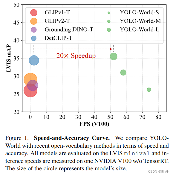
下表展现了YOLO-world在LVIS数据集上的zero-shot能力,可见效果优于当前Sota,但速度更快(评估硬件:NVIDIA V100 GPU w/o TensorRT)。

3.2 预训练数据集对效果的影响
用Object365和GlodG就能达到较好的效果。加入CC3M效果提升不是很大,可能是因为CC3M的标签是用2.3.1节的方法生成的,含有较多噪声导致。

3.3 text encoder对效果的影响
如果用轻量backbone最好结合微调。CLIP本身预训练的数据规模特别大,如果微调数据不多的话,frozen的效果反而好。


![[深度学习] 卷积神经网络“卷“在哪里?](https://img-blog.csdnimg.cn/direct/c795844a43de450fb266fccf030b6414.jpeg)