🌞欢迎来到PyTorch的世界
🌈博客主页:卿云阁💌欢迎关注🎉点赞👍收藏⭐️留言📝
🌟本文由卿云阁原创!
📆首发时间:🌹2024年2月16日🌹
✉️希望可以和大家一起完成进阶之路!
🙏作者水平很有限,如果发现错误,请留言轰炸哦!万分感谢!
目录
中间层优化2:Batch Normalization 批标准化和学习率衰减
输入端优化1---数据增强&数据归一化
为啥要进行数据增强
如何进行数据增强
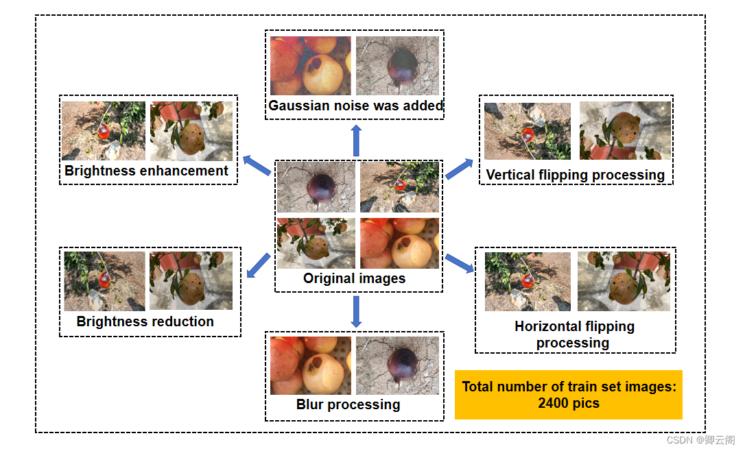
(2)数据增强效果(石榴缺陷为例)
注意事项
- 原始数据的多样性,比如同一类别不同个体、不同尺寸、不同角度等,原始数据的多样性对数据增强更有意义。
- 根据项目任务特点选择合适的数据增强方式,不合适的数据增强会对模型性能提升起到相反作用比如若任务为人脸识别,图像竖立翻转不应用于数据增强,因为不会出现倒立的情况。
数据归一化
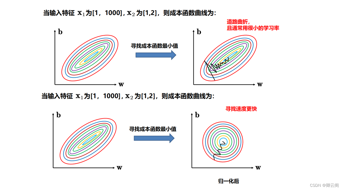
为啥要归一化
- 稳定性和收敛速度: 归一化可以使输入特征的范围在一个相对小的区间内,有助于优化算法更快地收敛。
- 避免梯度消失或梯度爆炸: 归一化有助于避免深层神经网络中的梯度消失或梯度爆炸问题,提高模型的稳定性。
- 提高模型泛化能力: 归一化可以帮助模型更好地泛化到新的未见数据,因为模型在训练时对输入特征的缩放不敏感。
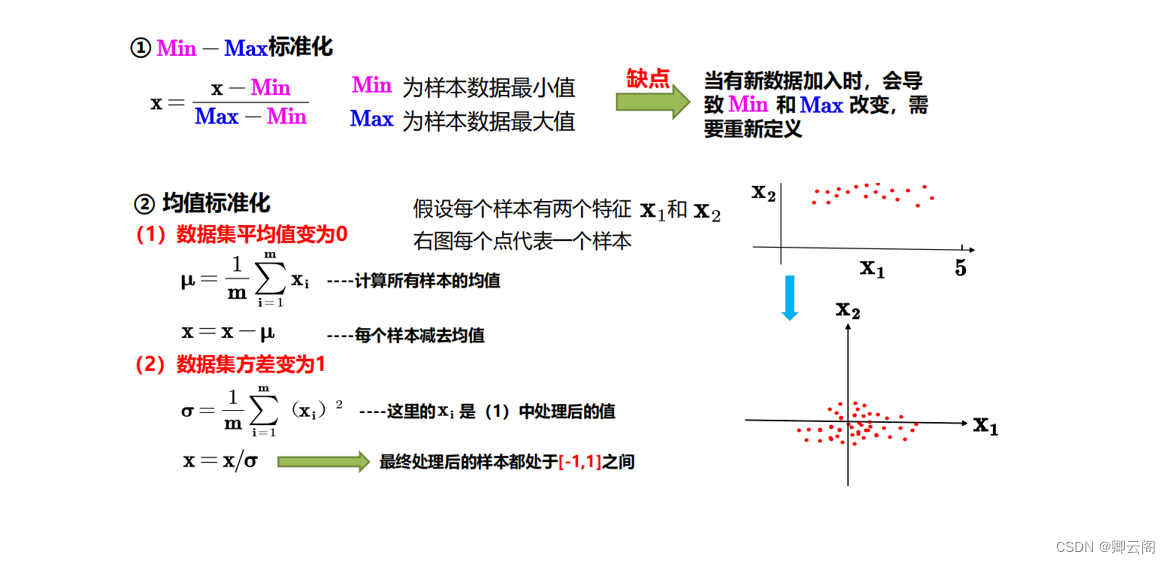
如何归一化
注意事项:
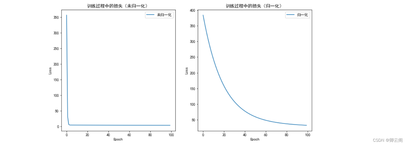
代码实现:
import torch
import torch.nn as nn
import torch.optim as optim
import matplotlib.pyplot as plt
from sklearn.preprocessing import MinMaxScaler
# 设置中文编码和负号的正常显示
plt.rcParams['font.sans-serif'] = ['SimHei']
plt.rcParams['axes.unicode_minus'] = False
# 生成一些随机数据
torch.manual_seed(42)
x_data = torch.rand(100, 1) * 10
y_data = 3 * x_data + 2 + torch.randn(100, 1) * 2

# 数据归一化
scaler = MinMaxScaler()
x_data_normalized = scaler.fit_transform(x_data)

# 定义线性回归模型
class LinearRegression(nn.Module):
    def __init__(self):
        super(LinearRegression, self).__init__()
        self.linear = nn.Linear(1, 1)

    def forward(self, x):
        return self.linear(x)

# 训练模型的函数
def train_model(model, x, y, epochs, lr):
    criterion = nn.MSELoss()
    optimizer = optim.SGD(model.parameters(), lr=lr)

    loss_list = []

    for epoch in range(epochs):
        y_pred = model(x)
        loss = criterion(y_pred, y)

        optimizer.zero_grad()
        loss.backward()
        optimizer.step()

        loss_list.append(loss.item())

    return loss_list

# 训练未归一化的模型
model_unnormalized = LinearRegression()
loss_list_unnormalized = train_model(model_unnormalized, x_data, y_data, epochs=100, lr=0.01)

# 训练归一化后的模型
model_normalized = LinearRegression()
loss_list_normalized = train_model(model_normalized, torch.tensor(x_data_normalized, dtype=torch.float32), y_data, epochs=100, lr=0.01)

# 可视化训练过程
plt.figure(figsize=(12, 6))

plt.subplot(1, 2, 1)
plt.plot(loss_list_unnormalized, label='未归一化')
plt.title('训练过程中的损失(未归一化)')
plt.xlabel('Epoch')
plt.ylabel('Loss')
plt.legend()

plt.subplot(1, 2, 2)
plt.plot(loss_list_normalized, label='归一化')
plt.title('训练过程中的损失(归一化)')
plt.xlabel('Epoch')
plt.ylabel('Loss')
plt.legend()

plt.show()
上图,我们的例子中好像没有归一化的效果要更好,究竟归一化的效果好不好还是要具体情况具体分析的哈。
输入端优化2:Mini-Batch梯度下降
中间层优化1:激活函数
为什么要用激活函数
每个神经元之间传输都用到激活函数,如果没有激活函数,一层神经网络和几百几千层神经网络都是一样的!加入激活函数,非线性曲线,只要网络层次多,可以解决非常复杂的分类,将神经网络成功激活。
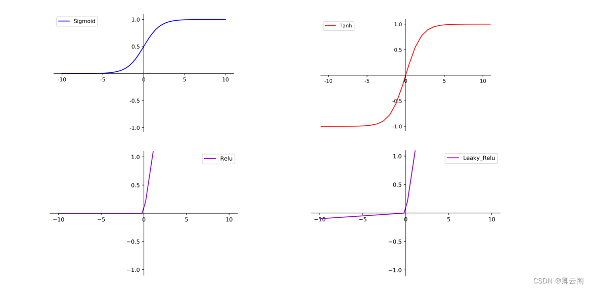
常见的激活函数
激活函数如何选择
- 不同的项目具体分析: 少批量数据训练,查看收敛效果
- 常用方式: Relu函数最多,Leaky_Relu函数少一些,二分类任务的输出层可采用sigmoid函数
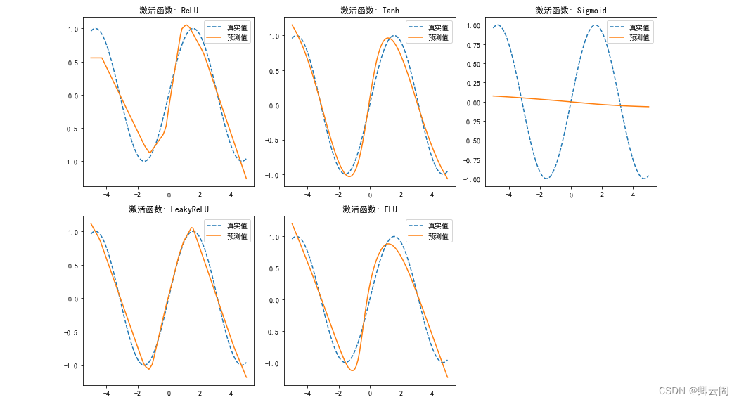
代码实现:
import torch
import torch.nn as nn
import torch.optim as optim
import matplotlib.pyplot as plt

# 生成一些随机数据
torch.manual_seed(42)
x_data = torch.linspace(-5, 5, 100).view(-1, 1)
y_true = torch.sin(x_data)

# 定义神经网络模型
class NeuralNetwork(nn.Module):
    def __init__(self, input_size, hidden_size, output_size, activation_function):
        super(NeuralNetwork, self).__init__()
        self.layer1 = nn.Linear(input_size, hidden_size)
        self.layer2 = nn.Linear(hidden_size, hidden_size)
        self.layer3 = nn.Linear(hidden_size, output_size)
        self.activation_function = activation_function

    def forward(self, x):
        x = self.activation_function(self.layer1(x))
        x = self.activation_function(self.layer2(x))
        x = self.layer3(x)
        return x

# 训练神经网络模型的函数
def train_model(model, x, y, epochs, lr):
    criterion = nn.MSELoss()
    optimizer = optim.SGD(model.parameters(), lr=lr)

    loss_list = []

    for epoch in range(epochs):
        y_pred = model(x)
        loss = criterion(y_pred, y)

        optimizer.zero_grad()
        loss.backward()
        optimizer.step()

        loss_list.append(loss.item())

    return loss_list

# 定义不同激活函数
activation_functions = [
    nn.ReLU(),
    nn.Tanh(),
    nn.Sigmoid(),
    nn.LeakyReLU(0.1),
    nn.ELU(),
]

# 可视化不同激活函数的输出
plt.figure(figsize=(12, 8))

for i, activation_function in enumerate(activation_functions, 1):
    model = NeuralNetwork(1, 10, 1, activation_function)
    loss_list = train_model(model, x_data, y_true, epochs=1000, lr=0.01)

    plt.subplot(2, 3, i)
    plt.plot(x_data.numpy(), y_true.numpy(), label='真实值', linestyle='dashed')
    plt.plot(x_data.numpy(), model(x_data).detach().numpy(), label='预测值')
    plt.title(f'激活函数: {type(activation_function).__name__}')
    plt.legend()

plt.tight_layout()
plt.show()
中间层优化2:Batch Normalization 批标准化和学习率衰减
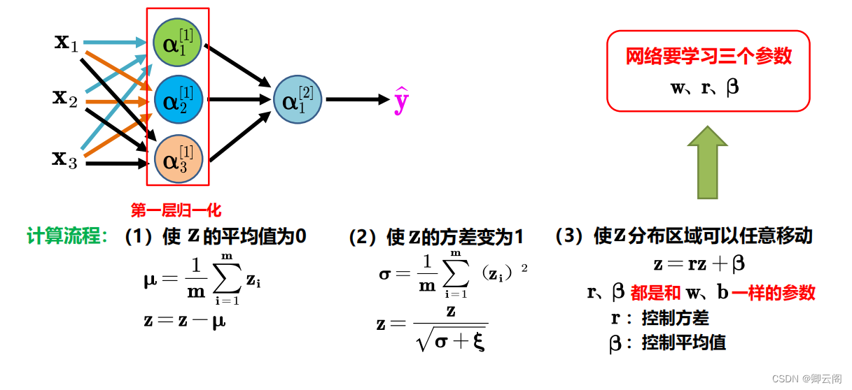
每层都做标准化
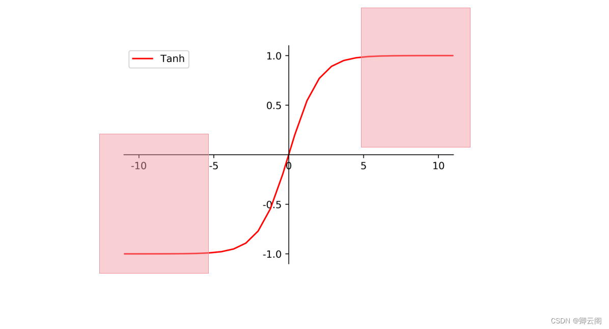
在神经网络中, 数据分布对训练会产生影响. 比如某个神经元 x 的值为1, 某个 Weights 的初始值为 0.1, 这样后一层神经元计算结果就是 Wx = 0.1; 又或者 x = 20, 这样 Wx 的结果就为 2. 现在还不能看出什么问题, 但是, 当我们加上一层激励函数, 激活这个 Wx 值的时候, 问题就来了. 如果使用 像 tanh 的激励函数, Wx 的激活值就变成了 ~0.1 和 ~1, 接近于 1 的部已经处在了 激励函数的饱和阶段, 也就是如果 x 无论再怎么扩大, tanh 激励函数输出值也还是 接近1. 换句话说, 神经网络在初始阶段已经不对那些比较大的 x 特征范围 敏感了. 这样很糟糕, 想象我轻轻拍自己的感觉和重重打自己的感觉居然没什么差别, 这就证明我的感官系统失效了. 当然我们是可以用之前提到的对数据做 normalization 预处理, 使得输入的 x 变化范围不会太大, 让输入值经过激励函数的敏感部分. 但刚刚这个不敏感问题不仅仅发生在神经网络的输入层, 而且在隐藏层中也经常会发生.只是时候 x 换到了隐藏层当中, 我们能不能对隐藏层的输入结果进行像之前那样的normalization 处理呢? 答案是可以的, 因为大牛们发明了一种技术, 叫做 batch normalization, 正是处理这种情况.
BN 算法
公式的后面还有一个反向操作, 将 normalize 后的数据再扩展和平移. 原来这是为了让神经网络自己去学着使用和修改这个扩展参数 gamma 𝛾, 和 平移参数 β, 这样神经网络就能自己慢慢琢磨出前面的 normalization 操作到底有没有起到优化的作用, 如果没有起到作用, 我就使用 gamma 𝛾 和 beta β 来抵消一些 normalization 的操作。
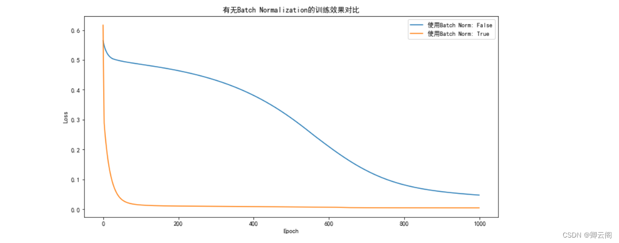
代码实现:
import torch
import torch.nn as nn
import torch.optim as optim
import matplotlib.pyplot as plt

# 生成一些随机数据
torch.manual_seed(42)
x_data = torch.linspace(-5, 5, 100).view(-1, 1)
y_true = torch.sin(x_data)

# 定义神经网络模型
class NeuralNetwork(nn.Module):
    def __init__(self, input_size, hidden_size, output_size, use_batch_norm=False):
        super(NeuralNetwork, self).__init__()
        self.layer1 = nn.Linear(input_size, hidden_size)
        self.layer2 = nn.Linear(hidden_size, hidden_size)
        self.layer3 = nn.Linear(hidden_size, output_size)
        self.use_batch_norm = use_batch_norm

        if self.use_batch_norm:
            self.batch_norm1 = nn.BatchNorm1d(hidden_size)
            self.batch_norm2 = nn.BatchNorm1d(hidden_size)

    def forward(self, x):
        x = torch.relu(self.layer1(x))

        if self.use_batch_norm:
            x = self.batch_norm1(x)

        x = torch.relu(self.layer2(x))

        if self.use_batch_norm:
            x = self.batch_norm2(x)

        x = self.layer3(x)
        return x

# 训练神经网络模型的函数
def train_model(model, x, y, epochs, lr):
    criterion = nn.MSELoss()
    optimizer = optim.SGD(model.parameters(), lr=lr)

    loss_list = []

    for epoch in range(epochs):
        y_pred = model(x)
        loss = criterion(y_pred, y)

        optimizer.zero_grad()
        loss.backward()
        optimizer.step()

        loss_list.append(loss.item())

    return loss_list

# 比较有无 Batch Normalization 的效果
plt.figure(figsize=(12, 6))

for use_batch_norm in [False, True]:
    model = NeuralNetwork(1, 10, 1, use_batch_norm)
    loss_list = train_model(model, x_data, y_true, epochs=1000, lr=0.01)

    plt.plot(loss_list, label=f'使用Batch Norm: {use_batch_norm}')

plt.title('有无Batch Normalization的训练效果对比')
plt.xlabel('Epoch')
plt.ylabel('Loss')
plt.legend()
plt.show()
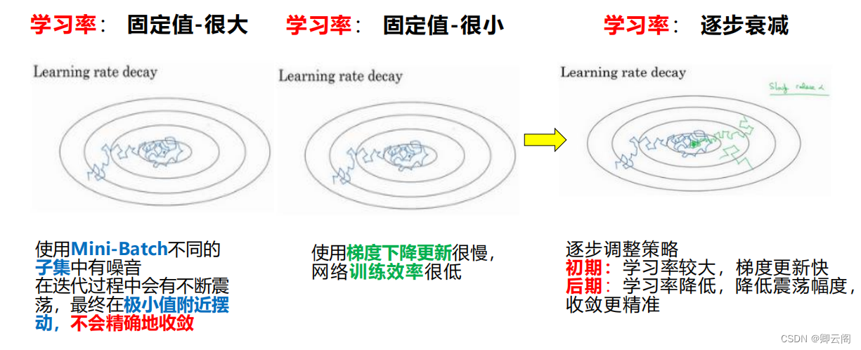
为什么要进行学习率衰减
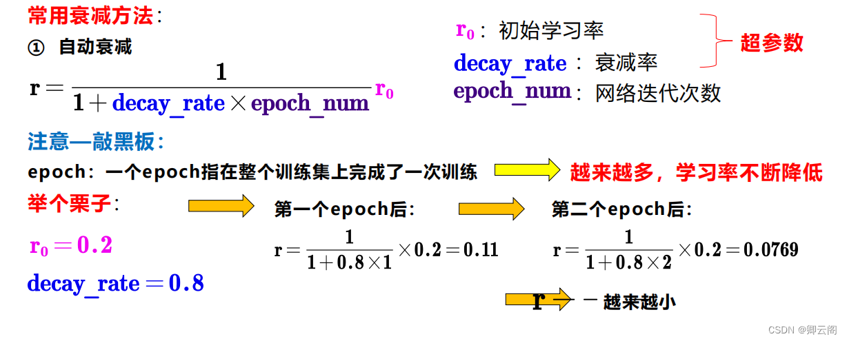
如何进行学习率衰减
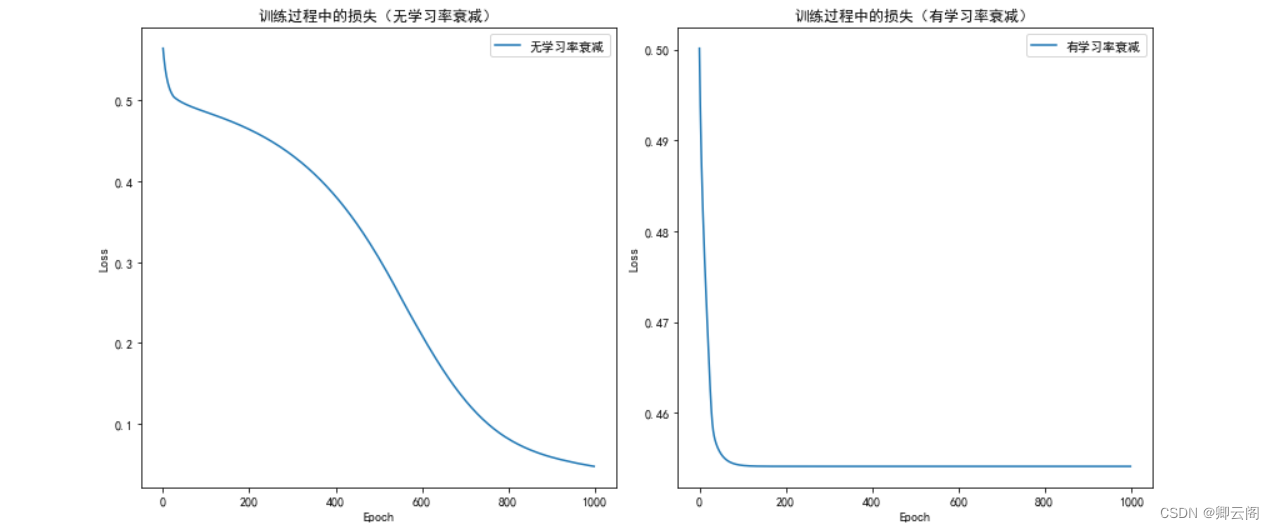
代码实现:
import torch
import torch.nn as nn
import torch.optim as optim
import matplotlib.pyplot as plt

# 生成一些随机数据
torch.manual_seed(42)
x_data = torch.linspace(-5, 5, 100).view(-1, 1)
y_true = torch.sin(x_data)

# 定义神经网络模型
class NeuralNetwork(nn.Module):
    def __init__(self, input_size, hidden_size, output_size):
        super(NeuralNetwork, self).__init__()
        self.layer1 = nn.Linear(input_size, hidden_size)
        self.layer2 = nn.Linear(hidden_size, hidden_size)
        self.layer3 = nn.Linear(hidden_size, output_size)

    def forward(self, x):
        x = torch.relu(self.layer1(x))
        x = torch.relu(self.layer2(x))
        x = self.layer3(x)
        return x

# 训练神经网络模型的函数
def train_model(model, x, y, epochs, lr, lr_decay=None):
    criterion = nn.MSELoss()
    optimizer = optim.SGD(model.parameters(), lr=lr)

    if lr_decay is not None:
        lr_scheduler = optim.lr_scheduler.ExponentialLR(optimizer, lr_decay)

    loss_list = []

    for epoch in range(epochs):
        y_pred = model(x)
        loss = criterion(y_pred, y)

        optimizer.zero_grad()
        loss.backward()
        optimizer.step()

        if lr_decay is not None:
            lr_scheduler.step()

        loss_list.append(loss.item())

    return loss_list

# 可视化有无学习率衰减的训练过程
plt.figure(figsize=(12, 6))

# 无学习率衰减
model_no_decay = NeuralNetwork(1, 10, 1)
loss_list_no_decay = train_model(model_no_decay, x_data, y_true, epochs=1000, lr=0.01, lr_decay=None)

# 有学习率衰减
model_decay = NeuralNetwork(1, 10, 1)
loss_list_decay = train_model(model_decay, x_data, y_true, epochs=1000, lr=0.01, lr_decay=0.95)

# 可视化
plt.subplot(1, 2, 1)
plt.plot(loss_list_no_decay, label='无学习率衰减')
plt.title('训练过程中的损失(无学习率衰减)')
plt.xlabel('Epoch')
plt.ylabel('Loss')
plt.legend()

plt.subplot(1, 2, 2)
plt.plot(loss_list_decay, label='有学习率衰减')
plt.title('训练过程中的损失(有学习率衰减)')
plt.xlabel('Epoch')
plt.ylabel('Loss')
plt.legend()

plt.tight_layout()
plt.show()
输出端优化1:softmax多分类器
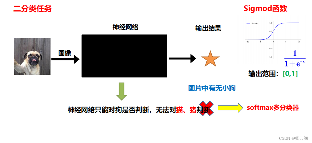
为什么要使用softmax多分类器?
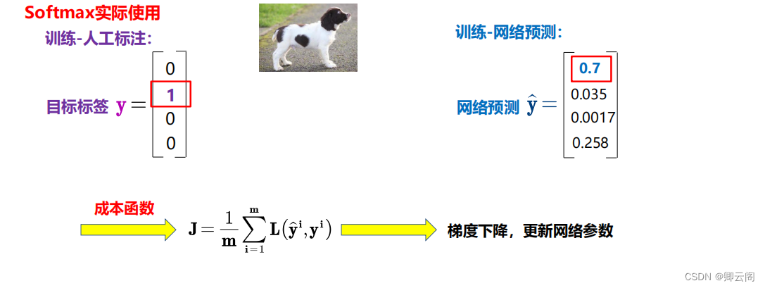
如何使用softmax多分类器?
代码实现:
import torch
import torch.nn as nn
import torch.optim as optim
from sklearn.datasets import load_iris
from sklearn.model_selection import train_test_split
import matplotlib.pyplot as plt
from sklearn.preprocessing import StandardScaler

# 加载Iris数据集
iris = load_iris()
X = iris.data
y = iris.target

# 数据预处理:标准化
scaler = StandardScaler()
X = scaler.fit_transform(X)

# 划分数据集
X_train, X_test, y_train, y_test = train_test_split(X, y, test_size=0.2, random_state=42)

# 转换为PyTorch的Tensor
X_train = torch.FloatTensor(X_train)
y_train = torch.LongTensor(y_train)
X_test = torch.FloatTensor(X_test)
y_test = torch.LongTensor(y_test)

# 定义神经网络模型
class NeuralNetwork(nn.Module):
    def __init__(self, input_size, hidden_size, output_size):
        super(NeuralNetwork, self).__init__()
        self.layer1 = nn.Linear(input_size, hidden_size)
        self.layer2 = nn.Linear(hidden_size, hidden_size)
        self.layer3 = nn.Linear(hidden_size, output_size)
        self.softmax = nn.Softmax(dim=1)

    def forward(self, x):
        x = torch.relu(self.layer1(x))
        x = torch.relu(self.layer2(x))
        x = self.layer3(x)
        x = self.softmax(x)
        return x

# 训练神经网络模型的函数
def train_model(model, X, y, epochs, lr):
    criterion = nn.CrossEntropyLoss()
    optimizer = optim.SGD(model.parameters(), lr=lr)

    loss_list = []

    for epoch in range(epochs):
        y_pred = model(X)
        loss = criterion(y_pred, y)

        optimizer.zero_grad()
        loss.backward()
        optimizer.step()

        loss_list.append(loss.item())

    return loss_list

# 创建并训练模型
input_size = X_train.shape[1]
output_size = len(torch.unique(y_train))
hidden_size = 10

model = NeuralNetwork(input_size, hidden_size, output_size)
loss_list = train_model(model, X_train, y_train, epochs=1000, lr=0.01)

# 可视化训练过程
plt.plot(loss_list)
plt.title('训练过程中的损失')
plt.xlabel('Epoch')
plt.ylabel('Loss')
plt.show()

# 在测试集上进行预测
with torch.no_grad():
    model.eval()
    y_pred_probs = model(X_test)
    y_pred = torch.argmax(y_pred_probs, dim=1)

# 可视化真实标签和预测标签的对比
plt.scatter(X_test[:, 0], X_test[:, 1], c=y_test, cmap='viridis', label='真实标签')
plt.scatter(X_test[:, 0], X_test[:, 1], c=y_pred, marker='x', cmap='viridis', label='预测标签')
plt.title('真实标签 vs 预测标签')
plt.xlabel('特征1')
plt.ylabel('特征2')
plt.legend()
plt.show()
训练过程的优化
训练结果的优化---过拟合 (Overfitting)
说白了, 就是机器学习模型于自信. 已经到了自负的阶段了. 那自负的坏处, 大家也知道, 就是在自己的小圈子里表现非凡, 不过在现实的大圈子里却往往处处碰壁. 所以在这个简介里, 我们把自负和过拟合画上等号.
如何解决:
方法一:
增加数据量, 大部分过拟合产生的原因是因为数据量太少了。
方法二:
运用正规化. L1, l2 regularization等等, 这些方法适用于大多数的机器学习, 包括神经网络. 他们的做法大同小异, 我们简化机器学习的关键公式为 y=Wx . W为机器需要学习到的各种参数. 在过拟合中, W 的值往往变化得特别大或特别小. 为了不让W变化太大, 我们在计算误差上做些手脚. 原始的 cost 误差是这样计算, cost = 预测值-真实值的平方. 如果 W 变得太大, 我们就让 cost 也跟着变大, 变成一种惩罚机制. 所以我们把 W 自己考虑进来. 这里 abs 是绝对值. 这一种形式的 正规化, 叫做 l1 正规化. L2 正规化和 l1 类似, 只是绝对值换成了平方. 其他的l3, l4 也都是换成了立方和4次方等等. 形式类似. 用这些方法,我们就能保证让学出来的线条不会过于扭曲.
import torch
import torch.nn as nn
import torch.optim as optim
import matplotlib.pyplot as plt

# 生成一些随机数据
torch.manual_seed(42)
x_data = torch.randn(100, 1) * 10
y_true = 3 * x_data + 2 + torch.randn(100, 1) * 2

# 定义神经网络模型
class NeuralNetwork(nn.Module):
    def __init__(self, input_size, hidden_size, output_size, regularization=None, reg_strength=0.01):
        super(NeuralNetwork, self).__init__()
        self.layer1 = nn.Linear(input_size, hidden_size)
        self.layer2 = nn.Linear(hidden_size, output_size)
        self.activation = nn.ReLU()
        self.regularization = regularization
        self.reg_strength = reg_strength

    def forward(self, x):
        x = self.activation(self.layer1(x))
        x = self.layer2(x)

        if self.regularization == 'l1':
            l1_penalty = self.reg_strength * torch.norm(self.layer1.weight, p=1)
            return x, l1_penalty
        elif self.regularization == 'l2':
            l2_penalty = self.reg_strength * torch.norm(self.layer1.weight, p=2)
            return x, l2_penalty
        else:
            return x

# 训练神经网络模型的函数
def train_model(model, x, y, epochs, lr):
    criterion = nn.MSELoss()
    optimizer = optim.SGD(model.parameters(), lr=lr)

    loss_list = []

    for epoch in range(epochs):
        if model.regularization:
            y_pred, penalty = model(x)
            loss = criterion(y_pred, y) + penalty
        else:
            y_pred = model(x)
            loss = criterion(y_pred, y)

        optimizer.zero_grad()
        loss.backward()
        optimizer.step()

        loss_list.append(loss.item())

    return loss_list

# 定义不同正则化方式
regularization_types = [None, 'l1', 'l2']

# 可视化不同正则化方式的效果
plt.figure(figsize=(12, 6))

for i, reg_type in enumerate(regularization_types, 1):
    model = NeuralNetwork(1, 10, 1, regularization=reg_type)
    loss_list = train_model(model, x_data, y_true, epochs=1000, lr=0.01)

    plt.subplot(1, 3, i)
    plt.plot(loss_list)
    plt.title(f'正则化方式: {reg_type if reg_type else "无"}')
    plt.xlabel('Epoch')
    plt.ylabel('Loss')

plt.tight_layout()
plt.show()
方法三:
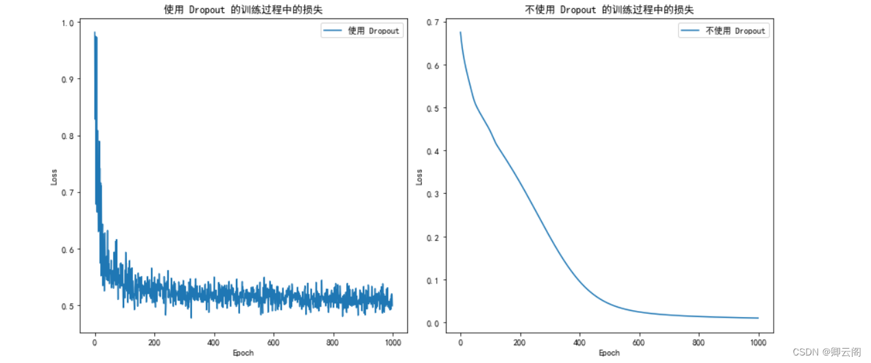
专门用在神经网络的正规化的方法, 叫作 dropout. 在训练的时候, 我们随机忽略掉一些神经元和神经联结 , 是这个神经网络变得”不完整”. 用一个不完整的神经网络训练一次.
到第二次再随机忽略另一些, 变成另一个不完整的神经网络. 有了这些随机 drop 掉的规则, 我们可以想象其实每次训练的时候, 我们都让每一次预测结果都不会依赖于其中某部分特定的神经元. 像l1, l2正规化一样, 过度依赖的 W , 也就是训练参数的数值会很大, l1, l2会惩罚这些大的 参数. Dropout 的做法是从根本上让神经网络没机会过度依赖.
import torch
import torch.nn as nn
import torch.optim as optim
import matplotlib.pyplot as plt

# 生成一些随机数据
torch.manual_seed(42)
x_data = torch.linspace(-5, 5, 100).view(-1, 1)
y_true = torch.sin(x_data)

# 定义神经网络模型
class NeuralNetwork(nn.Module):
    def __init__(self, input_size, hidden_size, output_size, use_dropout=False):
        super(NeuralNetwork, self).__init__()
        self.layer1 = nn.Linear(input_size, hidden_size)
        self.layer2 = nn.Linear(hidden_size, hidden_size)
        self.layer3 = nn.Linear(hidden_size, output_size)
        self.use_dropout = use_dropout

        # 如果使用 Dropout,添加 Dropout 层
        if self.use_dropout:
            self.dropout = nn.Dropout(p=0.5)

    def forward(self, x):
        x = torch.relu(self.layer1(x))

        # 如果使用 Dropout,应用 Dropout 操作
        if self.use_dropout:
            x = self.dropout(x)

        x = torch.relu(self.layer2(x))

        # 如果使用 Dropout,应用 Dropout 操作
        if self.use_dropout:
            x = self.dropout(x)

        x = self.layer3(x)
        return x

# 训练神经网络模型的函数
def train_model(model, x, y, epochs, lr):
    criterion = nn.MSELoss()
    optimizer = optim.SGD(model.parameters(), lr=lr)

    loss_list = []

    for epoch in range(epochs):
        y_pred = model(x)
        loss = criterion(y_pred, y)

        optimizer.zero_grad()
        loss.backward()
        optimizer.step()

        loss_list.append(loss.item())

    return loss_list

# 使用 Dropout 的模型
model_with_dropout = NeuralNetwork(1, 10, 1, use_dropout=True)
loss_list_with_dropout = train_model(model_with_dropout, x_data, y_true, epochs=1000, lr=0.01)

# 不使用 Dropout 的模型
model_without_dropout = NeuralNetwork(1, 10, 1, use_dropout=False)
loss_list_without_dropout = train_model(model_without_dropout, x_data, y_true, epochs=1000, lr=0.01)

# 可视化训练过程中的损失
plt.figure(figsize=(12, 6))

plt.subplot(1, 2, 1)
plt.plot(loss_list_with_dropout, label='使用 Dropout')
plt.title('使用 Dropout 的训练过程中的损失')
plt.xlabel('Epoch')
plt.ylabel('Loss')
plt.legend()

plt.subplot(1, 2, 2)
plt.plot(loss_list_without_dropout, label='不使用 Dropout')
plt.title('不使用 Dropout 的训练过程中的损失')
plt.xlabel('Epoch')
plt.ylabel('Loss')
plt.legend()

plt.tight_layout()
plt.show()


【Deep Learning 2】神经网络的优化
2024-02-16 15:04:01 29 阅读