【解决（几乎）任何机器学习问题】：超参数优化篇（超详细）

这篇文章相当长，您可以添加至收藏夹，以便在后续有空时候悠闲地阅读。

有了优秀的模型，就有了优化超参数以获得最佳得分模型的难题。那么，什么是超参数优化呢？假设您的机器学习项⽬有⼀个简单的流程。有⼀个数据集，你直接应⽤⼀个模型，然后得到结果。模型在这⾥的参数被称为超参数，即控制模型训练/拟合过程的参数。如果我们⽤ SGD 训练线性回归，模型的参数是斜率和偏差，超参数是学习率。你会发现我在本章和本书中交替使⽤这些术语。假设模型中有三个参数 a、b、c，所有这些参数都可以是 1 到 10 之间的整数。这些参数的 "正确 "组合将为您提供最佳结果。因此，这就有点像⼀个装有三拨密码锁的⼿提箱。不过，三拨密码锁只有⼀个正确答案。⽽模型有很多正确答案。那么，如何找到最佳参数呢？⼀种⽅法是对所有组合进⾏评估，看哪种组合能提⾼指标。让我们看看如何做到这⼀点。

best_accuracy = 0
best_parameters = {"a": 0, "b": 0, "c": 0}
for a in range(1, 11):
    for b in range(1, 11):
        for c in range(1, 11):
            model = MODEL(a, b, c)
            model.fit(training_data)
            preds = model.predict(validation_data)
            accuracy = metrics.accuracy_score(targets, preds)
            if accuracy > best_accuracy:
                best_accuracy = accuracy
                best_parameters["a"] = a
                best_parameters["b"] = b
                best_parameters["c"] = c

在上述代码中，我们从 1 到 10 对所有参数进⾏了拟合。因此，我们总共要对模型进⾏ 1000 次（10 x 10 x 10）拟合。这可能会很昂贵，因为模型的训练需要很⻓时间。不过，在这种情况下应该没问题，但在现实世界中，并不是只有三个参数，每个参数也不是只有⼗个值。⼤多数模型参数都是实数，不同参数的组合可以是⽆限的。

让我们看看 scikit-learn 的随机森林模型。

RandomForestClassifier(
    n_estimators=100,
    criterion='gini',
    max_depth=None,
    min_samples_split=2,
    min_samples_leaf=1,
    min_weight_fraction_leaf=0.0,
    max_features='auto',
    max_leaf_nodes=None,
    min_impurity_decrease=0.0,
    min_impurity_split=None,
    bootstrap=True,
    oob_score=False,
    n_jobs=None,
    random_state=None,
    verbose=0,
    warm_start=False,
    class_weight=None,
    ccp_alpha=0.0,
    max_samples=None,
    )

有 19 个参数，⽽所有这些参数的所有组合，以及它们可以承担的所有值，都将是⽆穷⽆尽的。通常情况下，我们没有⾜够的资源和时间来做这件事。因此，我们指定了⼀个参数⽹格。在这个⽹格上寻找最佳参数组合的搜索称为⽹格搜索。我们可以说，n_estimators 可以是 100、200、250、300、400、500；max_depth 可以是 1、2、5、7、11、15；criterion 可以是 gini 或 entropy。这些参数看起来并不多，但如果数据集过⼤，计算起来会耗费⼤量时间。我们可以像之前⼀样创建三个 for 循环，并在验证集上计算得分，这样就能实现⽹格搜索。还必须注意的是，如果要进⾏ k 折交叉验证，则需要更多的循环，这意味着需要更多的时间来找到完美的参数。因此，⽹格搜索并不流⾏。让我们以根据⼿机配置预测⼿机价格范围数据集为例，看看它是如何实现的。

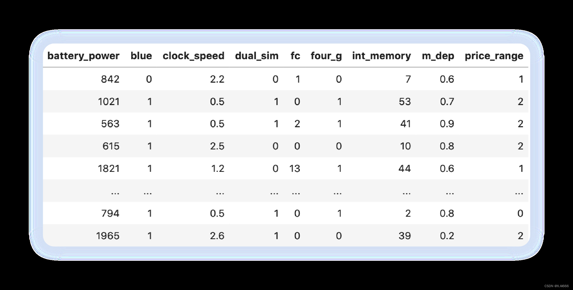
图 1 ：⼿机配置预测⼿机价格范围数据集展⽰

训练集中只有 2000 个样本。我们可以轻松地使⽤分层 kfold 和准确率作为评估指标。我们将使⽤具有上述参数范围的随机森林模型，并在下⾯的⽰例中了解如何进⾏⽹格搜索。

# rf_grid_search.py
import numpy as np
import pandas as pd
from sklearn import ensemble
from sklearn import metrics
from sklearn import model_selection

if __name__ == "__main__":
    df = pd.read_csv("./input/mobile_train.csv")
    X = df.drop("price_range", axis=1).values
    y = df.price_range.values

    classifier = ensemble.RandomForestClassifier(n_jobs=-1)
    param_grid = {
        "n_estimators": [100, 200, 250, 300, 400, 500],
        "max_depth": [1, 2, 5, 7, 11, 15],
        "criterion": ["gini", "entropy"]
    }

    model = model_selection.GridSearchCV(
        estimator=classifier,
        param_grid=param_grid,
        scoring="accuracy",
        verbose=10,
        n_jobs=1,
        cv=5
    )

    model.fit(X, y)
    print(f"Best score: {model.best_score_}")
    print("Best parameters set:")
    best_parameters = model.best_estimator_.get_params()
    for param_name in sorted(param_grid.keys()):
        print(f"\t{param_name}: {best_parameters[param_name]}")

这⾥打印了很多内容，让我们看看最后⼏⾏。

[ CV ] criterion = entropy , max_depth = 15 , n_estimators = 500 , score = 0.895 ,

total = 1.0 s

[ CV ] criterion = entropy , max_depth = 15 , n_estimators = 500 ...............

[ CV ] criterion = entropy , max_depth = 15 , n_estimators = 500 , score = 0.890 ,

total = 1.1 s

[ CV ] criterion = entropy , max_depth = 15 , n_estimators = 500 ...............

[ CV ] criterion = entropy , max_depth = 15 , n_estimators = 500 , score = 0.910 ,

total = 1.1 s

[ CV ] criterion = entropy , max_depth = 15 , n_estimators = 500 ...............

[ CV ] criterion = entropy , max_depth = 15 , n_estimators = 500 , score = 0.880 ,

total = 1.1 s

[ CV ] criterion = entropy , max_depth = 15 , n_estimators = 500 ...............

[ CV ] criterion = entropy , max_depth = 15 , n_estimators = 500 , score = 0.870 , total = 1.1 s

[ Parallel ( n_jobs = 1 )]: Done 360 out of 360 | elapsed : 3.7 min finished

Best score : 0.889

Best parameters set :

criterion : 'entropy'

max_depth : 15

n_estimators : 500

最后，我们可以看到，5折交叉检验最佳得分是 0.889，我们的⽹格搜索得到了最佳参数。我们可以使⽤的下⼀个最佳⽅法是随机搜索。在随机搜索中，我们随机选择⼀个参数组合，然后计算交叉验证得分。这⾥消耗的时间⽐⽹格搜索少，因为我们不对所有不同的参数组合进⾏评估。我们选择要对模型进⾏多少次评估，这就决定了搜索所需的时间。代码与上⾯的差别不⼤。除了GridSearchCV 外，我们使⽤ RandomizedSearchCV。

if __name__ == "__main__":
    classifier = ensemble.RandomForestClassifier(n_jobs=-1)
    param_grid = {
        "n_estimators": np.arange(100, 1500, 100),
        "max_depth": np.arange(1, 31),
        "criterion": ["gini", "entropy"]
    }
    model = model_selection.RandomizedSearchCV(
        estimator=classifier,
        param_distributions=param_grid,
        n_iter=20,
        scoring="accuracy",
        verbose=10,
        n_jobs=1,
        cv=5
    )
    model.fit(X, y)
    print(f"Best score: {model.best_score_}")
    print("Best parameters set:")
    best_parameters = model.best_estimator_.get_params()
    for param_name in sorted(param_grid.keys()):
        print(f"\t{param_name}: {best_parameters[param_name]}")

我们更改了随机搜索的参数⽹格，结果似乎有了些许改进。

Best score : 0.8905

Best parameters set :

criterion : entropy

max_depth : 25

n_estimators : 300

如果迭代次数较少，随机搜索⽐⽹格搜索更快。使⽤这两种⽅法，你可以为各种模型找到最优参数，只要它们有拟合和预测功能，这也是 scikit-learn 的标准。有时，你可能想使⽤管道。例如假设我们正在处理⼀个多类分类问题。在这个问题中，训练数据由两列⽂本组成，你需要建⽴⼀个模型来预测类别。让我们假设你选择的管道是⾸先以半监督的⽅式应⽤ tf-idf，然后使⽤SVD 和SVM 分类器。现在的问题是，我们必须选择 SVD 的成分，还需要调整 SVM 的参数。下⾯的代段展⽰了如何做到这⼀点。

import numpy as np
import pandas as pd
from sklearn import metrics
from sklearn import model_selection
from sklearn import pipeline
from sklearn.decomposition import TruncatedSVD
from sklearn.feature_extraction.text import TfidfVectorizer
from sklearn.preprocessing import StandardScaler
from sklearn.svm import SVC

def quadratic_weighted_kappa(y_true, y_pred):
    return metrics.cohen_kappa_score(y_true, y_pred, weights="quadratic")

if __name__ == '__main__':
    train = pd.read_csv('./input/train.csv')
    idx = test.id.values.astype(int)
    train = train.drop('id', axis=1)
    test = test.drop('id', axis=1)

    y = train.relevance.values
    traindata = list(train.apply(lambda x:'%s %s' % (x['text1'], x['text2']), axis=1))
    testdata = list(test.apply(lambda x:'%s %s' % (x['text1'], x['text2']), axis=1))

    tfv = TfidfVectorizer(
        min_df=3,
        max_features=None,
        strip_accents='unicode',
        analyzer='word',
        token_pattern=r'\w{1,}',
        ngram_range=(1, 3),
        use_idf=1,
        smooth_idf=1,
        sublinear_tf=1,
        stop_words='english'
    )

    tfv.fit(traindata)
    X = tfv.transform(traindata)
    X_test = tfv.transform(testdata)

    svd = TruncatedSVD()
    scl = StandardScaler()
    svm_model = SVC()

    clf = pipeline.Pipeline([
        ('svd', svd),
        ('scl', scl),
        ('svm', svm_model)
    ])

    param_grid = {
        'svd__n_components': [200, 300],
        'svm__C': [10, 12]
    }

    kappa_scorer = metrics.make_scorer(
        quadratic_weighted_kappa,
        greater_is_better=True
    )

    model = model_selection.GridSearchCV(
        estimator=clf,
        param_grid=param_grid,
        scoring=kappa_scorer,
        verbose=10,
        n_jobs=-1,
        refit=True,
        cv=5
    )

    model.fit(X, y)
    print("Best score: %0.3f" % model.best_score_)
    print("Best parameters set:")
    best_parameters = model.best_estimator_.get_params()
    for param_name in sorted(param_grid.keys()):
        print("\t%s: %r" % (param_name, best_parameters[param_name]))

    best_model = model.best_estimator_
    best_model.fit(X, y)
    preds = best_model.predict(X_test)

这⾥显⽰的管道包括 SVD（奇异值分解）、标准缩放和 SVM（⽀持向量机）模型。请注意，由于没有训练数据，您⽆法按原样运⾏上述代码。当我们进⼊⾼级超参数优化技术时，我们可以使⽤不同类型的最⼩化算法来研究函数的最⼩化。这可以通过使⽤多种最⼩化函数来实现，如下坡单纯形算法、内尔德-梅德优化算法、使⽤⻉叶斯技术和⾼斯过程寻找最优参数或使⽤遗传算法。我将在 "集合与堆叠（ensembling and stacking） "⼀章中详细介绍下坡单纯形算法和 NelderMead 算法的应⽤。⾸先，让我们看看⾼斯过程如何⽤于超参数优化。这类算法需要⼀个可以优化的函数。⼤多数情况下，都是最⼩化这个函数，就像我们最⼩化损失⼀样。因此，⽐⽅说，你想找到最佳参数以获得最佳准确度，显然，准确度越⾼越好。现在，我们不能最⼩化精确度，但我们可以将精确度乘以-1。这样，我们是在最⼩化精确度的负值，但事实上，我们是在最⼤化精确度。在⾼斯过程中使⽤⻉叶斯优化，可以使⽤ scikit-optimize (skopt) 库中的 gp_minimize 函数。让我们看看如何使⽤该函数调整随机森林模型的参数。

# rf_gp_minimize.py
import numpy as np
import pandas as pd
from functools import partial
from sklearn import ensemble
from sklearn import metrics
from sklearn import model_selection
from skopt import gp_minimize
from skopt import space

def optimize(params, param_names, x, y):
    params = dict(zip(param_names, params))
    model = ensemble.RandomForestClassifier(**params)
    kf = model_selection.StratifiedKFold(n_splits=5)
    accuracies = []

    for idx in kf.split(X=x, y=y):
        train_idx, test_idx = idx[0], idx[1]
        xtrain = x[train_idx]
        ytrain = y[train_idx]
        xtest = x[test_idx]
        ytest = y[test_idx]

        model.fit(xtrain, ytrain)
        preds = model.predict(xtest)
        fold_accuracy = metrics.accuracy_score(ytest, preds)
        accuracies.append(fold_accuracy)

    return -1 * np.mean(accuracies)

if __name__ == "__main__":
    df = pd.read_csv("./input/mobile_train.csv")
    X = df.drop("price_range", axis=1).values
    y = df.price_range.values

    param_space = [
        space.Integer(3, 15, name="max_depth"),
        space.Integer(100, 1500, name="n_estimators"),
        space.Categorical(["gini", "entropy"], name="criterion"),
        space.Real(0.01, 1, prior="uniform", name="max_features")
    ]

    param_names = [
        "max_depth",
        "n_estimators",
        "criterion",
        "max_features"
    ]

    optimization_function = partial(
        optimize,
        param_names=param_names,
        x=X,
        y=y
    )

    result = gp_minimize(
        optimization_function,
        dimensions=param_space,
        n_calls=15,
        n_random_starts=10,
        verbose=10
    )

    best_params = dict(
        zip(
            param_names,
            result.x
        )
    )
    print(best_params)

这同样会产⽣⼤量输出，最后⼀部分如下所⽰。

Iteration No : 14 started . Searching for the next optimal point .

Iteration No : 14 ended . Search finished for the next optimal point .

Time taken : 4.7793

Function value obtained : - 0.9075

Current minimum : - 0.9075

Iteration No : 15 started . Searching for the next optimal point .

Iteration No : 15 ended . Search finished for the next optimal point .

Time taken : 49.4186

Function value obtained : - 0.9075

Current minimum : - 0.9075

{ 'max_depth' : 12 , 'n_estimators' : 100 , 'criterion' : 'entropy' ,

'max_features' : 1.0 }

看来我们已经成功突破了 0.90的准确率。这真是太神奇了！

我们还可以通过以下代码段查看（绘制）我们是如何实现收敛的。

from skopt . plots import plot_convergence

plot_convergence ( result )

收敛图如图 2 所⽰。

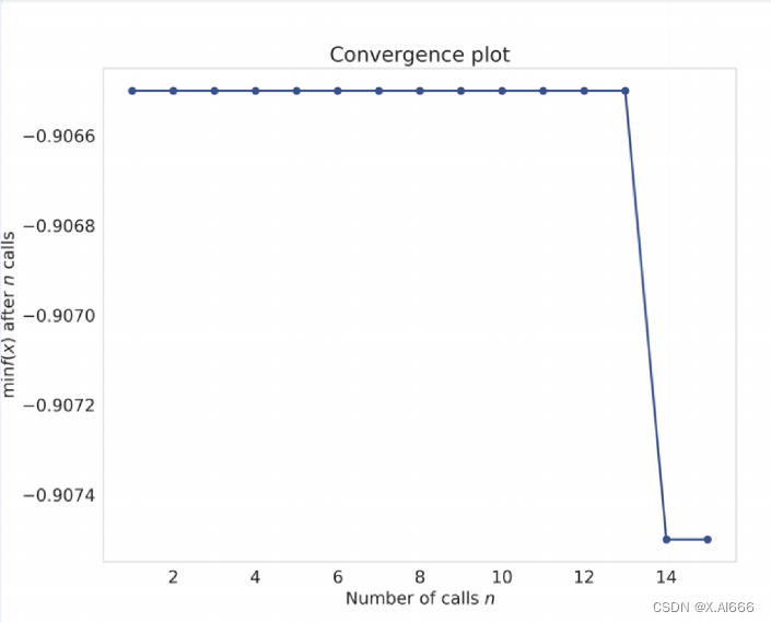
图 2：随机森林参数优化的收敛图

Scikit- optimize 就是这样⼀个库。 hyperopt 使⽤树状结构帕岑估计器（TPE）来找到最优参数。请看下⾯的代码⽚段，我在使⽤ hyperopt 时对之前的代码做了最⼩的改动。

import numpy as np
import pandas as pd
from functools import partial
from sklearn import ensemble
from sklearn import metrics
from sklearn import model_selection
from hyperopt import hp, fmin, tpe, Trials
from hyperopt.pyll.base import scope

def optimize(params, x, y):
    model = ensemble.RandomForestClassifier(**params)
    kf = model_selection.StratifiedKFold(n_splits=5)
    accuracies = []

    for idx in kf.split(X=x, y=y):
        train_idx, test_idx = idx[0], idx[1]
        xtrain = x[train_idx]
        ytrain = y[train_idx]
        xtest = x[test_idx]
        ytest = y[test_idx]

        model.fit(xtrain, ytrain)
        preds = model.predict(xtest)
        fold_accuracy = metrics.accuracy_score(ytest, preds)
        accuracies.append(fold_accuracy)

    return -1 * np.mean(accuracies)

if __name__ == "__main__":
    df = pd.read_csv("./input/mobile_train.csv")
    X = df.drop("price_range", axis=1).values
    y = df.price_range.values

    param_space = {
        "max_depth": scope.int(hp.quniform("max_depth", 1, 15, 1)),
        "n_estimators": scope.int(hp.quniform("n_estimators", 100, 1500, 1)),
        "criterion": hp.choice("criterion", ["gini", "entropy"]),
        "max_features": hp.uniform("max_features", 0, 1)
    }

    optimization_function = partial(
        optimize,
        x=X,
        y=y
    )

    trials = Trials()
    hopt = fmin(
        fn=optimization_function,
        space=param_space,
        algo=tpe.suggest,
        max_evals=15,
        trials=trials
    )

    print(hopt)

正如你所看到的，这与之前的代码并⽆太⼤区别。你必须以不同的格式定义参数空间，还需要改

变实际优化部分，⽤ hyperopt 代替 gp_minimize。结果相当不错！

❯ python rf_hyperopt . py

100 %| ██████████████████ | 15 / 15 [ 0 4 : 38 < 0 0 : 0 0 , 18.57 s / trial , best loss : -

0.9095000000000001 ]

{ 'criterion' : 1 , 'max_depth' : 11.0 , 'max_features' : 0.821163568049807 ,

'n_estimators' : 806.0 }

我们得到了⽐以前更好的准确度和⼀组可以使⽤的参数。请注意，最终结果中的标准是 1。这意味着选择了 1，即熵。上述调整超参数的⽅法是最常⻅的，⼏乎适⽤于所有模型：线性回归、逻辑回归、基于树的⽅法、梯度提升模型（如 xgboost、lightgbm），甚⾄神经⽹络！

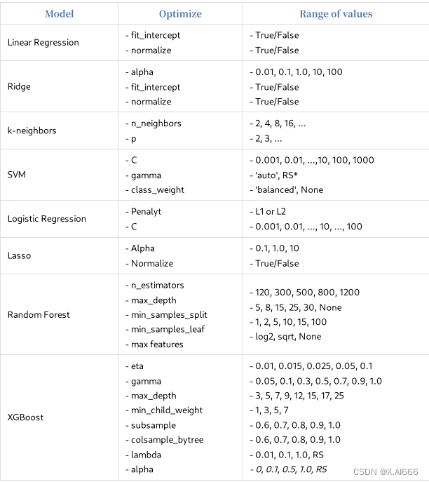
虽然这些⽅法已经存在，但学习时必须从⼿动调整超参数开始，即⼿⼯调整。⼿动调整可以帮助你学习基础知识，例如，在梯度提升中，当你增加深度时，你应该降低学习率。如果使⽤⾃动⼯具，就⽆法学习到这⼀点。请参考下表，了解应如何调整。RS* 表⽰随机搜索应该更好.

⼀旦你能更好地⼿动调整参数，你甚⾄可能不需要任何⾃动超参数调整。创建⼤型模型或引⼊⼤量特征时，也容易造成训练数据的过度拟合。为避免过度拟合，需要在训练数据特征中引⼊噪声或对代价函数进⾏惩罚。这种惩罚称为正则化，有助于泛化模型。在线性模型中，最常⻅的正则化类型是 L1 和 L2。L1 也称为 Lasso 回归，L2 称为 Ridge 回归。说到神经⽹络，我们会使⽤ dropout、添加增强、噪声等⽅法对模型进⾏正则化。利⽤超参数优化，还可以找到正确的惩罚⽅法。

【解决（几乎）任何机器学习问题】：超参数优化篇（超详细）

相关推荐

最近更新

热门阅读