机器学习 | KNN算法 - 酸梨子-专注技术分享

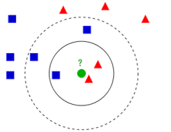
一、KNN算法核心思想和原理

1.1、怎么想出来的？

近朱者赤，近墨者黑！

距离决定一切、民主集中制

1.2、基本原理 —— 分类

k个最近的邻居
民主集中制投票
分类表决与加权分类表决

1.3、基本原理 —— 回归

计算未知点的值
决策规则不同
均值法与加权均值法

1.4、如何选择K值？

K太小导致“过拟合”（过分相信某个数据），容易把噪声学进来
K太大导致“欠拟合”，决策效率低

K不能太小也不能太大
Fit = 最优拟合（找三五个熟悉的人问问），通过超参数调参实现 ~

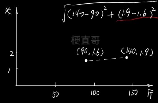
1.5、距离的度量

明氏距离 Minkowski Distance
- p为距离的阶数，n为特征空间的维度
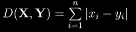
- p=1时，即曼哈顿距离；p=2时，即欧式距离
- p趋向于无穷时，为切比雪夫距离
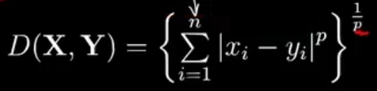
·p=1时，曼哈顿距离 Manhattan Distance
·p=2时，欧式距离 Euclidean Distance
- 空间中两点的直线距离

1.6、特征归一化的重要性

简单来讲，就是统一坐标轴比例

二、代码实现

KNN 预测的过程

1. 计算新样本点与已知样本点的距离

2. 按距离排序

3. 确定k值

4. 距离最近的k个点投票

若不使用scikit-learn:

import numpy as np
import matplotlib.pyplot as plt
from collections import Counter

# 样本特征
data_X = [
    [1.3, 6],
    [3.5, 5],
    [4.2, 2],
    [5, 3.3],
    [2, 9],
    [5, 7.5],
    [7.2, 4 ],
    [8.1, 8],
    [9, 2.5]
]
# 样本标记
data_y = [0,0,0,0,1,1,1,1,1]
# 训练集
X_train = np.array(data_X)
y_train = np.array(data_y)
# 新的样本点
data_new = np.array([4,5])

# 1. 计算新样本点与已知样本点的距离
distance = [np.sqrt(np.sum(data - data_new)**2) for data in X_train]
# 2. 按距离排序
sort_index = np.argsort(distance)
# 3. 确定k值
k = 5
# 4. 距离最近的k个点投票
first_k = [y_train[i] for i in sort_index[:k]]
predict_y = Counter(first_k).most_common(1)[0][0]

print(predict_y)

若使用sklearn：

import numpy as np
from sklearn.neighbors import KNeighborsClassifier

# 样本特征
data_X = [
    [1.3, 6],
    [3.5, 5],
    [4.2, 2],
    [5, 3.3],
    [2, 9],
    [5, 7.5],
    [7.2, 4 ],
    [8.1, 8],
    [9, 2.5]
]
# 样本标记
data_y = [0,0,0,0,1,1,1,1,1]
# 训练集
X_train = np.array(data_X)
y_train = np.array(data_y)
# 新的样本点
data_new = np.array([4,5])

# 创造类的实例
knn_classifier = KNeighborsClassifier(n_neighbors=5)
# fit
knn_classifier.fit(X_train,y_train)
# sklearn支持预测多个数据，而我们只有一个数据，所以需要将其转为二维
data_new.reshape(1,-1)
predict_y = knn_classifier.predict(data_new.reshape(1,-1))

print(predict_y)

三、划分数据集：训练集与预测集

为什么要划分数据集？

评价模型性能

防止过拟合

提升泛化能力

3.1、划分数据集代码实现

import numpy as np 
from matplotlib import pyplot as plt
from sklearn.datasets import make_blobs

x, y = make_blobs(
    n_samples = 300, # 样本总数
    n_features = 2,
    centers = 3,
    cluster_std = 1, # 类內标准差
    center_box = (-10, 10),
    random_state = 233, 
    return_centers = False
)

plt.scatter(x[:,0], x[:,1], c = y,s = 15)
plt.show()

划分数据集

index = np.arange(20)

index

array([ 0,  1,  2,  3,  4,  5,  6,  7,  8,  9, 10, 11, 12, 13, 14, 15, 16,
       17, 18, 19])

np.random.shuffle(index)

index

array([13, 16,  2, 19,  7, 14,  9,  0,  1, 11,  8,  6, 15, 10,  4, 18,  3,
       12, 17,  5])

np.random.permutation(20)

array([12, 19,  6,  7, 11, 10,  4,  8, 16,  3,  2, 15, 18,  5,  9,  0,  1,
       14, 13, 17])

np.random.seed(233)
shuffle = np.random.permutation(len(x))

shuffle

array([ 23,  86, 204, 287, 206, 170, 234,  94, 146, 180, 263,  22,   3,
       264, 194, 290, 229, 177, 208, 202,  10, 188, 262, 120, 148, 121,
        98, 160, 267, 136, 294,   2,  34, 142, 271, 133, 127,  12,  29,
        49, 112, 218,  36,  57,  45,  11,  25, 151, 212, 289, 157,  19,
       275, 176, 144,  82, 161,  77,  51, 152, 135,  16,  65, 189, 298,
       279,  37, 187,  44, 210, 178, 165,   6, 162,  66,  32, 198,  43,
       108, 211,  67, 119, 284,  90,  89,  56, 217, 158, 228, 248, 191,
        47, 296, 123, 181, 200,  40,  87, 232,  97, 113, 122, 220, 153,
       173,  68,  99,  61, 273, 269, 281, 209,   4, 110, 259,  95, 205,
       288,   8, 283, 231, 291, 171, 111, 242, 216, 285,  54, 100,  38,
       185, 235, 174, 201, 107, 223, 222, 196, 268, 114, 147, 166,  85,
        39,  58, 256, 258,  74, 251,  15, 150, 137,  70,  91,  52,  14,
       169,  21, 184, 207, 238, 128, 219, 125, 293, 134,  27, 265,  96,
       270,  18, 109, 126, 203,  88, 249,  92, 213,  60, 227,   5,  59,
         9, 138, 236, 280, 124, 199, 225, 149, 145, 246, 192, 102,  48,
        73,  20,  31,  63, 237,  78,  62, 233, 118, 277,  28,  50,  64,
       117, 197, 140,   7, 105, 252,  71, 190,  76, 103,  93, 183,  72,
         0, 278,  79, 172, 214, 182, 292, 139, 260,  30, 195,  13, 244,
       240, 297, 257, 245, 143, 186, 243, 266, 286, 168, 179,  81, 215,
       129, 167, 106, 261,  42, 276,  69, 224, 253, 247, 155, 154,  17,
       132,  24, 141, 239,  80, 101,  75, 159, 116,  46, 272, 226,  83,
       156,  33, 115, 282, 299,  55, 250, 221, 254, 255,  41, 130, 104,
        26,  53,  84, 274,   1, 163, 230,  35, 241, 164, 193, 175, 131,
       295])

shuffle.shape

(300,)

train_size = 0.7

train_index = shuffle[:int(len(x) * train_size)]

test_index = shuffle[int(len(x) * train_size):]

train_index.shape, test_index.shape

((210,), (90,))

x[train_index].shape, y[train_index].shape

((210, 2), (210,))

x[test_index].shape, y[test_index].shape

((90, 2), (90,))

def my_train_test_split(x, y, train_size = 0.7, random_state = None):
    if random_state:
        np.random.seed(random_state)
    shuffle = np.random.permutation(len(x))
    train_index = shuffle[:int(len(x) * train_size)]
    test_index = shuffle[int(len(x) * train_size):]
    return x[train_index], x[test_index], y[train_index], y[test_index]

x_train, x_test, y_train, y_test = my_train_test_split(x, y, train_size = 0.7, random_state = 233)

x_train.shape, x_test.shape, y_train.shape, y_test.shape

((210, 2), (90, 2), (210,), (90,))

plt.scatter(x_train[:, 0], x_train[:, 1], c = y_train, s = 15)
plt.show()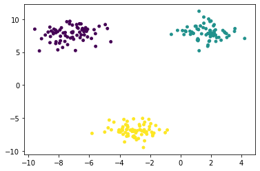

plt.scatter(x_test[:, 0], x_test[:, 1], c = y_test, s = 15)
plt.show()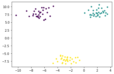

3.2、sklearn划分数据集

from sklearn.model_selection import train_test_split

x_train, x_test, y_train, y_test = train_test_split(x, y, train_size = 0.7, random_state = 233)

x_train.shape, x_test.shape, y_train.shape, y_test.shape

((210, 2), (90, 2), (210,), (90,))

from collections import Counter
Counter(y_test)

Counter({2: 34, 0: 25, 1: 31})

x_train, x_test, y_train, y_test = train_test_split(x, y, train_size = 0.7, random_state = 233, stratify = y)

Counter(y_test)

Counter({2: 30, 0: 30, 1: 30})

四、模型评价

import numpy as np
from sklearn import datasets
from sklearn.model_selection import train_test_split
from sklearn.neighbors import KNeighborsClassifier
from sklearn.metrics import accuracy_score

# 1、加载数据集
iris = datasets.load_iris()
X = iris.data
y = iris.target

# 2、拆分数据集,首先需乱序处理
# 2.1、自己拆分不调包 ~
shuffle_index = np.random.permutation(len(y))
train_ratio = 0.8
train_size = int(len(y)*train_ratio)
train_index = shuffle_index[:train_size]
test_index = shuffle_index[train_size:]

X_train = X[train_index]
y_train = y[train_index]

X_test = X[test_index]
y_test = y[test_index]

# 2.2、调包 ~
X_train, X_test, y_train, y_test = train_test_split(X,y,train_size=0.8,random_state=666)

# 3、预测
knn_classifier = KNeighborsClassifier(n_neighbors=5)
knn_classifier.fit(X_train, y_train)
# 若不关注预测结果只关注预测精度
# accuracy_score(X_test,y_test)
y_predict = knn_classifier.predict(X_test)
print(y_predict)

# 4、评价
accutacy = np.sum(y_predict == y_test) / len(y_test)
# 或使用
accuracy_score(y_test,y_predict)

五、超参数 Hyperpatameter

人为设置的参数 / 经验值 / 参数搜索

KNN的三个超参数：

k个最近的邻居

分类表决与加权分类表决

明氏距离中的p

首先加载数据

import numpy as np
from sklearn.model_selection import train_test_split
from sklearn.datasets import load_iris

iris = load_iris()

x = iris.data
y = iris.target

x.shape, y.shape

((150, 4), (150,))

x_train, x_test, y_train, y_test = train_test_split(x, y, train_size=0.7, random_state=233, stratify=y)

x_train.shape, x_test.shape, y_train.shape, y_test.shape

((105, 4), (45, 4), (105,), (45,))

5.1、超参数

from sklearn.neighbors import KNeighborsClassifier

neigh = KNeighborsClassifier(
    n_neighbors=3,
    weights='distance',#'uniform',
    p = 2
)

neigh.fit(x_train, y_train)

KNeighborsClassifier

KNeighborsClassifier(n_neighbors=3, weights='distance')

neigh.score(x_test, y_test)

0.9777777777777777

best_score = -1
best_n  = -1
best_weight = ''
best_p = -1

for n in range(1, 20):
    for weight in ['uniform', 'distance']:
        for p in range(1, 7):
            neigh = KNeighborsClassifier(
                n_neighbors=n,
                weights=weight,
                p = p
            )
            neigh.fit(x_train, y_train)
            score = neigh.score(x_test, y_test)
            
            if score > best_score:
                best_score = score
                best_n = n
                best_weight = weight
                best_p = p

print("n_neighbors:", best_n)
print("weights:", best_weight)
print("p:", best_p)
print("score:", best_score)

n_neighbors: 5
weights: uniform
p: 2
score: 1.0

5.2、sklearn 超参数搜索

from sklearn.model_selection import GridSearchCV

params = {
    'n_neighbors': [n for n in range(1, 20)],
    'weights': ['uniform', 'distance'],
    'p': [p for p in range(1, 7)]
}

grid = GridSearchCV(
    estimator=KNeighborsClassifier(),
    param_grid=params,
    n_jobs=-1
)

grid.fit(x_train, y_train)

GridSearchCV

GridSearchCV(estimator=KNeighborsClassifier(), n_jobs=-1,
             param_grid={'n_neighbors': [1, 2, 3, 4, 5, 6, 7, 8, 9, 10, 11, 12,
                                         13, 14, 15, 16, 17, 18, 19],
                         'p': [1, 2, 3, 4, 5, 6],
                         'weights': ['uniform', 'distance']})

estimator: KNeighborsClassifier

KNeighborsClassifier()

KNeighborsClassifier

KNeighborsClassifier()

grid.best_params_

{'n_neighbors': 9, 'p': 2, 'weights': 'uniform'}

grid.best_score_

0.961904761904762

grid.best_estimator_

KNeighborsClassifier

KNeighborsClassifier(n_neighbors=9)

grid.best_estimator_.predict(x_test)

array([2, 2, 0, 1, 1, 1, 2, 0, 2, 0, 0, 1, 0, 2, 1, 1, 0, 2, 2, 1, 0, 1,
       1, 2, 2, 0, 0, 1, 1, 0, 2, 2, 0, 1, 1, 2, 1, 1, 0, 0, 0, 2, 0, 1,
       1])

grid.best_estimator_.score(x_test, y_test)

0.9555555555555556

六、特征归一化

特征量纲不同。为了消除数据特征量纲之间的影响，使得不同指标具有一定程度的可比性，能够同时反应每个指标的重要程度。

6.1、最值归一化方法

适用于数据分布在有限范围的情况。但受特殊数值影响很大。

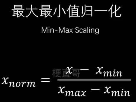
X[:,0] = (X[:,0] - np.min(X[:,0])) /  (np.max(X[:,0]) - np.min(X[:,0]))

X[:5,0]

array([0.22222222, 0.16666667, 0.11111111, 0.08333333, 0.19444444])

6.2、零均值归一化

X[:,0] = (X[:,0] - np.mean(X[:,0]))/np.std(X[:,0])

X[:5,0]

array([-0.90068117, -1.14301691, -1.38535265, -1.50652052, -1.02184904])

scikit-learn 中的StandardScaler

from sklearn.preprocessing import StandardScaler

standard_scaler = StandardScaler()

standard_scaler.fit(X)

standard_scaler.mean_

array([5.84333333, 3.05733333, 3.758     , 1.19933333])

standard_scaler.scale_

array([0.82530129, 0.43441097, 1.75940407, 0.75969263])

注意要重新赋值给X！

X = standard_scaler.transform(X)

** 测试集如何归一化？

不是用测试集的均值和标准差，而是用训练集的！

import numpy as np
from sklearn import datasets
from sklearn.model_selection import train_test_split
from sklearn.preprocessing import StandardScaler
from sklearn.neighbors import KNeighborsClassifier

iris = datasets.load_iris()
X_train,X_test,y_train,y_test = train_test_split(iris.data,iris.target,train_size=0.8,random_state=666)

standard_scaler = StandardScaler()
standard_scaler.fit(X_train)

X_train_standard = standard_scaler.transform(X_train)
X_test_standard = standard_scaler.transform(X_test)

knn_classifier = KNeighborsClassifier(n_neighbors=5)
knn_classifier.fit(X_train_standard,y_train)
knn_classifier.score(X_test_standard, y_test)

代码参考于

Chapter-04/4-7 特征归一化.ipynb · 梗直哥/Machine-Learning - Gitee.com