【手撕LLM-Medusa】并行解码范式：美杜萨驾到, 通通闪开!!

前言

美杜莎（希腊语：Μέδουσα；英语：Medusa）是古希腊神话中的蛇发女妖, 为何能将蛇法女妖和LLM解码联系起来呢？这便是我们今天要探究的主题Medusa Decoding

1. Introduction

Medusa: Simple LLM Inference Acceleration Framework with Multiple Decoding Heads

LLM最常见的Decoder-only Transfoemrs结构在解码时, 通常会串行逐个生成token ，如何并行解码是LLM推理加速中比较独特的方式。在过去有Speculative Decoding 能巧妙的实现“并行解码”，但解码过程需要有小模型(Draft Model)参与，使得工程实现和部署并不够优雅。

Medusa 则提供了一种One Model 的并行解码方案，其实现动机在于增加Multiple Decoding Heads 来做Next-Next-Token 预测，提高预测效率，这里的Heads 和美杜莎的形象不谋而合。

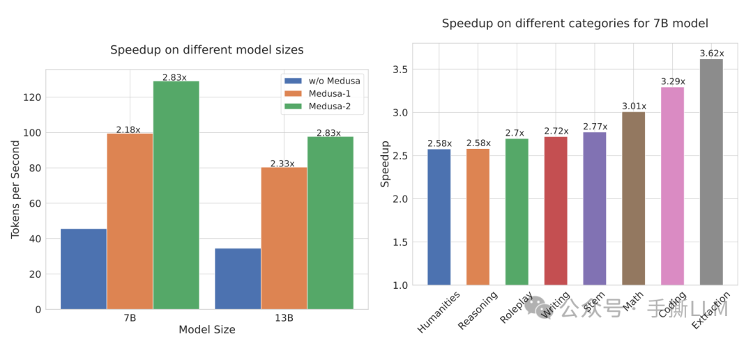
Medusa加速效果如下

相较baseline, Medusa-2 加速2.83x
在Math/Coding/Extraction 种类的推理任务中加速3x以上

带着以下问题来探究Medusa

Medusa 头是什么样的结构
Medusa 如何训练的？
Medusa 2 与1有什么区别
Medusa的解码步骤是怎么样的，为什么能边验证边生成
Medusa 是如何提高接收率的
什么是Tree Attenion Machanism, 候选解码路径如何生成, 多条解码路径如何确认最优解码路径
为什么要用Typical Acceptance
self-distillation 如何使得Medusa头输出分布能对齐模型
如何区分 Speculative Decoding、Medusa Decoding, LookAhead Decoding

2. Medusa

目前有Medusa1和Medusa2，两者在结构无区别，而Medusa2加入了更多训练技巧，提点明显7B模型从2.18x加速提升到2.83x

2.1 架构介绍

2.1.1 模型架构

通常将常规的decoding过程称为Next-Token 预测，将多token并行解码定义为Next-Next-Tokens 预测，统一任务形式。

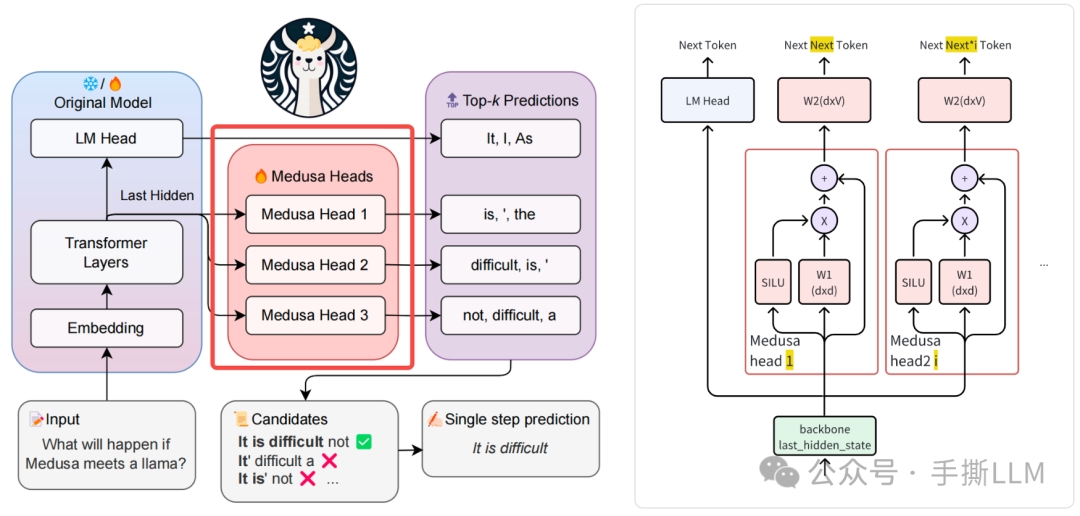
Medusa 在现有模型基础上，增加多个Medusa Head，与原模型上的LM Head 一同做预测。

新增的Medusa Head 包含Block(可以多个堆叠)和分类头，输入为backbone模型的Last Hidden数据，输出为预测Token的概率
原文有个typo，会做一次零初始化, 从原LM_head 来初始化保持输出分布一致

We initialize _W_1(k) identically to the original language model head, and _W_2(k) to zero
下图左边有3个medusa头，包含原LM_head模型一次性可以输出1+3个token

代码实现如下

# Medusa Block   class ResBlock(nn.Module):       def __init__(self, hidden_size):           super().__init__()           self.linear = nn.Linear(hidden_size, hidden_size) #W1           torch.nn.init.zeros_(self.linear.weight)           self.act = nn.SiLU()       def forward(self, x):           return x + self.act(self.linear(x))            # Medusa Model   class MedusaModel(nn.Module):       def __init__(           self, base_model, medusa_num_heads=4, medusa_num_layers=1,           base_model_name_or_path=None,       ):         	# LLM Model         	self.base_model = base_model           # Medusa Blocks and Medusa Heads           self.medusa_head = nn.ModuleList(               [                   nn.Sequential(                       *([ResBlock(self.hidden_size)] * medusa_num_layers),                       nn.Linear(self.hidden_size, self.vocab_size, bias=False), # W2 dxv                   )                   for _ in range(medusa_num_heads)               ]           )           # ...

初始化

model = MedusaModel(           llama_model,           medusa_num_heads=4,           medusa_num_layers=1,           base_model_name_or_path='./min_llama',       )   print(model.base_model.lm_head)   print(model.medusa_head)

输出打印

Linear(in_features=32, out_features=4, bias=False)   ModuleList(     (0-3): 4 x Sequential(       (0): ResBlock(         (linear): Linear(in_features=32, out_features=32, bias=True)         (act): SiLU()       )       (1): Linear(in_features=32, out_features=4, bias=False)     )   )

2.1.2 Medusa 1 训练

Medusa1在训练过程中会将原模型参数冻结， Medusa 头参数需要训练

设为位置的token，训练 Loss为:

This introduces a more democratized way to accelerate LLM inference, as with the quantization, MEDUSA can be trained for a large model on a single consumer GPU similar to QLoRA. The training only takes a few hours (e.g., 5 hours for MEDUSA-1 on Vicuna 7B model with a single NVIDIA A100 PCIE GPU to train on 60k ShareGPT samples).

由于仅有Medusa 头参数需要训练，则可以用QLoRA微调：

数据：ShareGPT (使用与Vicuna同样的训练数据)
耗时：5h A100x1
模型 : Vicuna 7B

常规的标签需要便宜点1个位置, 这里的labels[..., 2 + i :] , 由于不训练 LM Head，所以shift 2个位置

# medusa/train/train.py   def compute_loss(self, model, inputs, return_outputs=False):     logits = model(input_ids=inputs["input_ids"],                    attention_mask=inputs["attention_mask"])     labels = inputs["labels"]     loss = 0     # Shift so that tokens < n predict n     for i in range(medusa):         medusa_logits = logits[i, :, : -(2 + i)].contiguous()         medusa_labels = labels[..., 2 + i :].contiguous()         medusa_logits = medusa_logits.view(-1,logits.shape[-1])         medusa_labels = medusa_labels.view(-1)         medusa_labels = medusa_labels.to(medusa_logits.device)         loss_i = CrossEntropyLoss(medusa_logits, medusa_labels)         loss += loss_i

2.2 Medusa Decoding

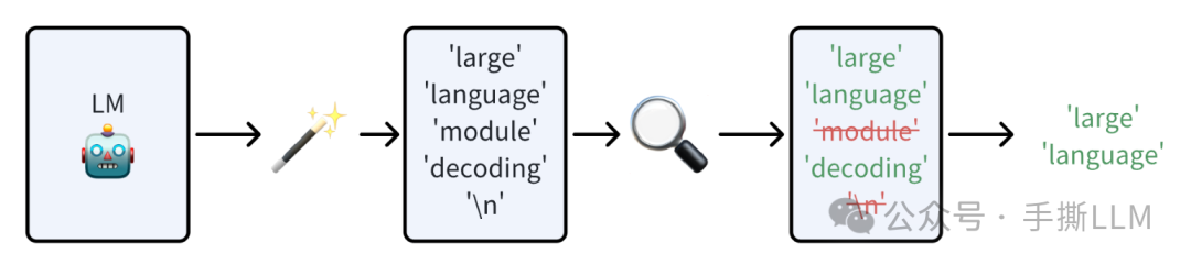
并行解码范式遵循两个流程

低成本的得到Next-Next-Token
将Next-Next-Token序列做一次verify

在Speculative Decoding 中, 使用 Draft model 来低成本获得Next-Next-Token , 而Medusa仅通过增加头层计算就能达到同样的效果

Medusa更大的优势在于，除了第一次Prefill外，后续可以达到边verify边生成的效果

2.2.1 Medusa Inference

在首次推理中，可以得到各个头的预测，但无法确认Medusa Head预测的token是否正确

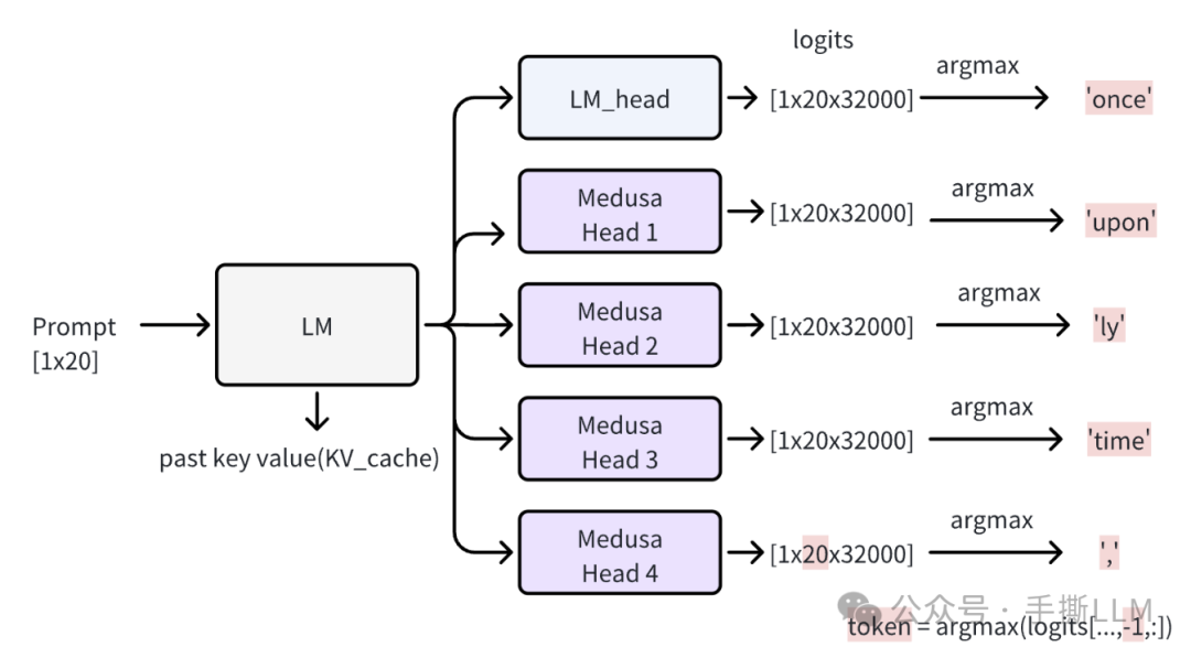
一次forward计算出各个头的logits

with torch.inference_mode():       input_ids = tokenizer([prompt]).input_ids       input_len = len(input_ids[0])       input_ids = torch.as_tensor(input_ids).cuda()       model.current_length_data.zero_() # this is for rerun       medusa_logits, outputs, logits = model(input_ids, output_orig = True, past_key_values=model.past_key_values)   print('Medusa logits shape:', medusa_logits.shape, 'logits shape:', logits.shape)

输出为

Medusa logits shape: torch.Size([4, 1, 20, 32000])    logits shape: torch.Size([1, 20, 32000])

取argmax得到各个头的所预测出的token

medusa_pred = torch.argmax(medusa_logits[..., -1, :], dim = -1)   pred = torch.argmax(logits[..., -1, :], dim = -1)   print('Base model prediction:', tokenizer.batch_decode(pred))   print('Medusa prediction:', tokenizer.batch_decode(medusa_pred))   preds = torch.cat([pred, medusa_pred[:, 0 ], dim = -1) # 将用于Verify   print('Combined prediction:', tokenizer.batch_decode(preds))

输出为

Base model prediction: ['Once']   Medusa prediction: ['upon', 'ly', 'time', ',']   Combined prediction: ['Once', 'upon', 'ly', 'time', ',']

2.2.2 Medusa Verify

在修正步骤中，包含三个步骤

借助past_key_value, 可以将第一次预测的5个token当成query与20个KV进行前向计算，经过softmax得到5个next token【绿色】
将5个next token与query错位校验，就能得出接受的token，如下图右上角得到accept_length为2的token。

a. 事实上仅有“upon”匹配上了，X[0] once-> y[0] upon = x[1] upon

b. 基于once, upon 预测出来的a是可以被接受的，不需要再错位校验。
最精髓的是Medusa Head会取accept length位置的token，当成是下一轮的输入

至此我们经过两轮forward 计算就得到了3个token, 那么加速为 3/2=1.5x, 综合步骤2和3，Medusa把verify和Next-Next-Token 一起做了，这是与Speculative Decoding 比较大的一个区别

我们将第一步推理结果preds进行修正，注意到以下代码

preds作为query, model.past_key_values 作为kv_cache 可以减少计算时间

with torch.inference_mode():     medusa_logits, outputs, logits = model(preds.cuda().unsqueeze(0), output_orig = True, past_key_values = model.past_key_values)

medusa_pred = torch.argmax(medusa_logits[..., -5:, :], dim = -1)   pred = torch.argmax(logits[..., :, :], dim = -1)   print('Base model prediction:', tokenizer.batch_decode(pred[0]))   print('truncated input tokens:', preds[1:].tolist())   print('Output tokens:', pred[0, :].tolist())

输出为

Base model prediction: ['upon', 'a', 'a', ',', 'in']   truncated input tokens: [2501, 368, 931, 29892]   Output tokens: [2501, 263, 263, 29892, 297]

校验过程

posterior_mask = (               preds[1:] == pred[0, :-1]           ).int() # 错位校验   accept_length = torch.cumprod(posterior_mask, dim = -1).sum().item() # 得到解码接受长度   cur_length = accept_length + input_len + 1   print('Posterior mask:', posterior_mask.tolist())   print('Accept length:', accept_length)   print('Current KV cache length for attention modules:', model.current_length_data[0].item())   print('Start length:', input_len, ',current length:', cur_length)   # update kv cache   model.current_length_data.fill_(cur_length)   # create new input   preds = torch.cat([pred[:, accept_length], medusa_pred[:,0,accept_length], dim = -1)   print('Combined prediction:', tokenizer.batch_decode(preds))

输出结果为

Posterior mask: [1, 0, 0, 1] # 一旦中途有0就拒不接受后面的预测   Accept length: 1   Current KV cache length for attention modules: 71   Start length: 66 ,current length: 68   Combined prediction: ['a', 'time', ',', 'there', 'a']

小结：verify过程只需要有past_key_value和preds，相当于第一次要需要做Prefill，之后就一直做verify就行了

2.2.3 past key Value 解析

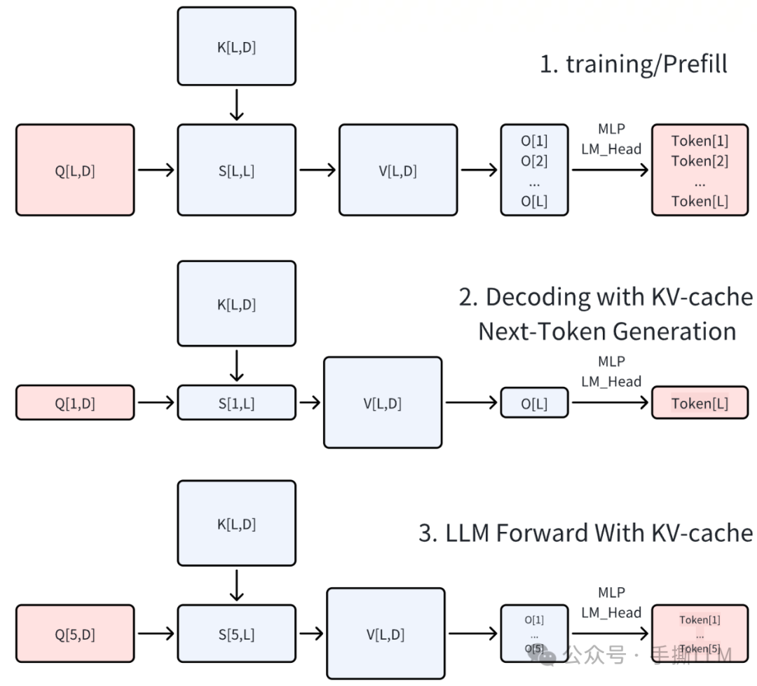
论文里提到的past key value 即是我们常说的KV-Cache

根据不同的Q 会有不同的输出张量,

上图为全Q、K、V，通常见于训练过程或Prefill过程
中图为存在KV-Cache时，仅输入最新的token作为Q就能做Next-Token预测
下图为输入批量的Q，那么得到批量的token预测，即是Medusa的Verify时的计算形式

2.3 小结

至此，我们已经剖析将 Medusa 的baseline的核心实现，颇见锋芒

新增的Medusa Head需要训练, 数据构造需要偏移>1位
Medusa 的推理流程可以理解：Prefill + Verify + Verify + …
这里的加速比1.5x是，我们接下来思考更精妙的优化技巧，使得并行解码的接受率更高

3. Tree Attention Mechanism

3.1 Introduction

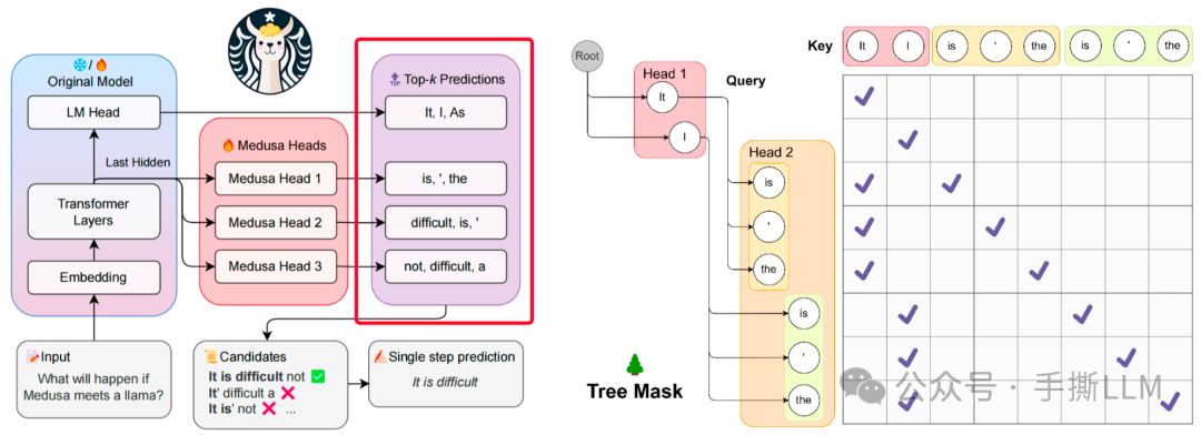
在Medusa中，上述的Medusa Head基础版本解码采用greedy方式取Top-1 Token，实际上可以在每个Medusa Head采用Top-k 得到多个候选token，构建出树状结构，LM_head 的输出作为根节点，树的深度自顶向下遍历称为解码路径(论文里用candidate path)。

图示右图存在6条解码路径，

[It, is],[It, '],[It, the],[I, is],[I, '],[I, the],

3.1.1 解码路径数量分析

LM-head 取Top-1， Medusa-head 取Top-k个tokens，假设共有4个头

Top-3: 候选路径有条
Top-10: 候选路径有条

可想, 解码路径会随着Top-k 和头数增多急剧增加，那么新的问题是

如何能减少候选解码路径？
如何能在候选解码路径中，得到最优解码路径？

3.2 Top-K 候选集

我们可以通过torch的top-k获取每个medusa头的top-k token预测，这里只有Medusa Head的输出才取top-k

import torch   TOPK = 3   medusa_logits = torch.randn([4, 1, 10, 32000])   candidates_medusa_logits = torch.topk(medusa_logits[:, 0, -1], 1, dim = -1).indices   print(candidates_medusa_logits)   candidates_medusa_logits = torch.topk(medusa_logits[:, 0, -1], TOPK, dim = -1).indices   print(candidates_medusa_logits)

输出为:

# 4个头top-1输出   tensor([[25300],           [15445],           [ 8174],           [13761])   # 4个头top-3输出   tensor([[25300,  8173,  9022],           [15445,  5827, 26862],           [ 8174, 16607, 30043],           [13761, 18943, 24824])

此时产生解码路径为, 罗列共有

[25300, 15545, 8172, 13761]
[25300, 15545, 8172, 18943]
[25300, 15545, 8172, 24824]
[25300, 15545, 16607, 13761]
…

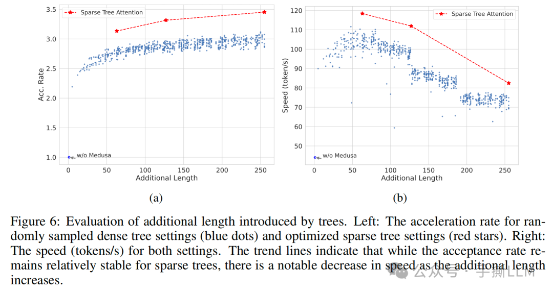
3.3 Sparse Tree Path

当Top-k 变大时，会产生大量的候选路径，具有庞大的搜索空间, 那么可以试着构造一种稀疏的树结构，能极具减少树搜索规模

Medusa在论文里举例了一种Top-10的稀疏树结构，是手动设计的。
第2层从左数第1号节点有10个子节点
第2层从左数第2号节点有7个子节点
第2层从左数第3号节点有3个子节点
树的层数时Medusa对应的头数-1，除掉Root
每一层的token的数量为Medusa的Top-k取值
手工设计的稀疏树结构，越靠前的节点，有更多的子节点路径，这样就较为合理的减枝条
这样就将1000个路径的树优化到只有42条路径(数叶子结点)
这里的路径可以提前结束，不要求一定要便利到最后一层

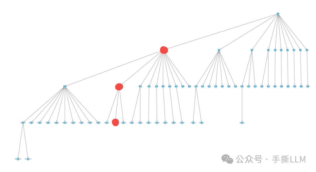
查看代码里的手工路径表，以上红点的路径为[0,1,1], 并且这条路线的长度可以不为4

[0,1,1] 第0个元素值为0，代表第1个medusa头top-k的token中取第0个token

# medusa/model/medusa_choices.py   mc_sim_7b_63 = [[0], [0, 0], [1], [0, 1], [2], [0, 0, 0], [1, 0], [0, 2], [3], [0, 3], [4], [0, 4], [2, 0], [0, 5], [0, 0, 1], [5], [0, 6], [6], [0, 7], [0, 1, 0], [1, 1], [7], [0, 8], [0, 0, 2], [3, 0], [0, 9], [8], [9], [1, 0, 0], [0, 2, 0], [1, 2], [0, 0, 3], [4, 0], [2, 1], [0, 0, 4], [0, 0, 5], [0, 0, 0, 0], [0, 1, 1], [0, 0, 6], [0, 3, 0], [5, 0], [1, 3], [0, 0, 7], [0, 0, 8], [0, 0, 9], [6, 0], [0, 4, 0], [1, 4], [7, 0], [0, 1, 2], [2, 0, 0], [3, 1], [2, 2], [8, 0], [0, 5, 0], [1, 5], [1, 0, 1], [0, 2, 1], [9, 0], [0, 6, 0], [0, 0, 0, 1], [1, 6], [0, 7, 0]

树状数据结构是由medusa_buffer来进行管理的，该实现的思想是做树数据结构的稀疏化管理

根据Medusa choies 我们可以构建稀疏树的所有数据成员,

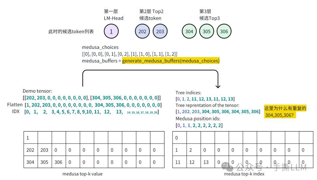
代码实现为

demo_tensor = torch.zeros(2,10).long() # top-k=10   demo_tensor[0,0] = 202   demo_tensor[0,1] = 203   demo_tensor[1,0] = 304   demo_tensor[1,1] = 305   demo_tensor[1,2] = 306   print('Demo tensor: \n', demo_tensor.tolist())   demo_tensor = demo_tensor.flatten()   demo_tensor = torch.cat([torch.ones(1).long(), demo_tensor])   print('Demo tensor flatten & cat:\n', demo_tensor.tolist())   print('='*50)   medusa_choices = [[0], [0, 0], [0, 1], [0, 2], [1], [1, 0], [1, 1], [1, 2]   medusa_buffers = generate_medusa_buffers(medusa_choices, device='cpu')   tree_indices = medusa_buffers['tree_indices']   medusa_position_ids = medusa_buffers['medusa_position_ids']   retrieve_indices = medusa_buffers['retrieve_indices']   print('Tree indices: \n', tree_indices.tolist())   print('Tree reprentation of the tensor: \n', demo_tensor[tree_indices].tolist())   print('='*50)   print('Medusa position ids: \n', medusa_position_ids.tolist())   print('='*50)   print('Retrieve indices: \n', retrieve_indices.tolist())   demo_tensor_tree = demo_tensor[tree_indices]   demo_tensor_tree_ext = torch.cat([demo_tensor_tree, torch.ones(1).long().mul(-1)])   print('Retrieve reprentation of the tensor: \n', demo_tensor_tree_ext[retrieve_indices].tolist())   print('='*50)      print(medusa_buffers['medusa_attn_mask'][0,0,:,:].int())

输出结果为

Demo tensor:    [[202, 203, 0, 0, 0, 0, 0, 0, 0, 0], [304, 305, 306, 0, 0, 0, 0, 0, 0, 0]   Demo tensor flatten & cat:   [1, 202, 203, 0, 0, 0, 0, 0, 0, 0, 0, 304, 305, 306, 0, 0, 0, 0, 0, 0, 0]   ==================================================   Tree indices:    [0, 1, 2, 11, 12, 13, 11, 12, 13]   Tree reprentation of the tensor:    [1, 202, 203, 304, 305, 306, 304, 305, 306]   ==================================================   Medusa position ids:    [0, 1, 1, 2, 2, 2, 2, 2, 2]   ==================================================   Retrieve indices:    [[0, 2, 8], [0, 2, 7], [0, 2, 6], [0, 1, 5], [0, 1, 4], [0, 1, 3]   Retrieve reprentation of the tensor:    [[1, 203, 306], [1, 203, 305], [1, 203, 304], [1, 202, 306], [1, 202, 305], [1, 202, 304]   ==================================================   tensor([[1, 0, 0, 0, 0, 0, 0, 0, 0],           [1, 1, 0, 0, 0, 0, 0, 0, 0],           [1, 0, 1, 0, 0, 0, 0, 0, 0],           [1, 1, 0, 1, 0, 0, 0, 0, 0],           [1, 1, 0, 0, 1, 0, 0, 0, 0],           [1, 1, 0, 0, 0, 1, 0, 0, 0],           [1, 0, 1, 0, 0, 0, 1, 0, 0],           [1, 0, 1, 0, 0, 0, 0, 1, 0],           [1, 0, 1, 0, 0, 0, 0, 0, 1], dtype=torch.int32)

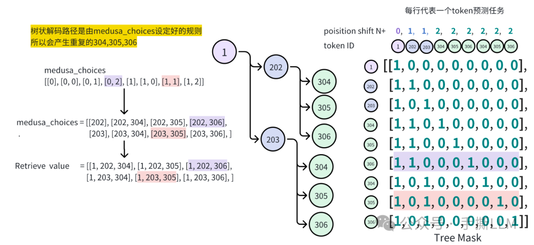
如下图解Tree Mask的由来和后续作用

Medusa choices决定解码路径，故将choices可视化成中间的树结构图
Mask矩阵的每行都可以代表一个token预测任务
在Tree Mask矩阵中，需要对位置编码进行错位编码

3.4 Tree Attention Mechanism实现细节

当引入树搜索结构后，需要重新组织generate代码结构，核心包含6个步骤

generate_medusa_buffers : 根据设定的medusa choices得到稀疏的树结构表达
initialize_medusa: 首次预填充past_key_value, 便于后续verify
generate_candidates : 生成候选路径
tree_decoding : 基于tree mask每行计算logits
evaluate_posterior: 评估每条路径合理性
update_inference_inputs: 更新kv cache，preds

# medusa/model/medusa_model_legacy.py   def medusa_generate(         self,         ....     ):          # 1. 根据设定的medusa choices得到稀疏的树结构表达       medusa_buffers = generate_medusa_buffers(                 medusa_choices, device=self.base_model.device             )          reset_medusa_mode(self)          # 2. 首次预填充past_key_value, 便于后续verify       # Initialize tree attention mask and process prefill tokens       medusa_logits, logits = initialize_medusa(           input_ids, self, medusa_buffers["medusa_attn_mask"], past_key_values       )          new_token = 0       last_round_token = 0          for idx in range(max_steps):              # 3. 生成候选路径           candidates, tree_candidates = generate_candidates(               # ...           )                      # 4. 基于tree mask每行计算logits           medusa_logits, logits, outputs = tree_decoding(               #...           )                      # reordering logits           logits = tree_logits[0, medusa_buffers["retrieve_indices"]           medusa_logits = tree_medusa_logits[:, 0, medusa_buffers["retrieve_indices"]                      # 5. 评估每条路径合理性           best_candidate, accept_length = evaluate_posterior(               #...           )      				# 6. 更新kv cache，preds           input_ids, logits, medusa_logits, new_token = update_inference_inputs(               ##....           )

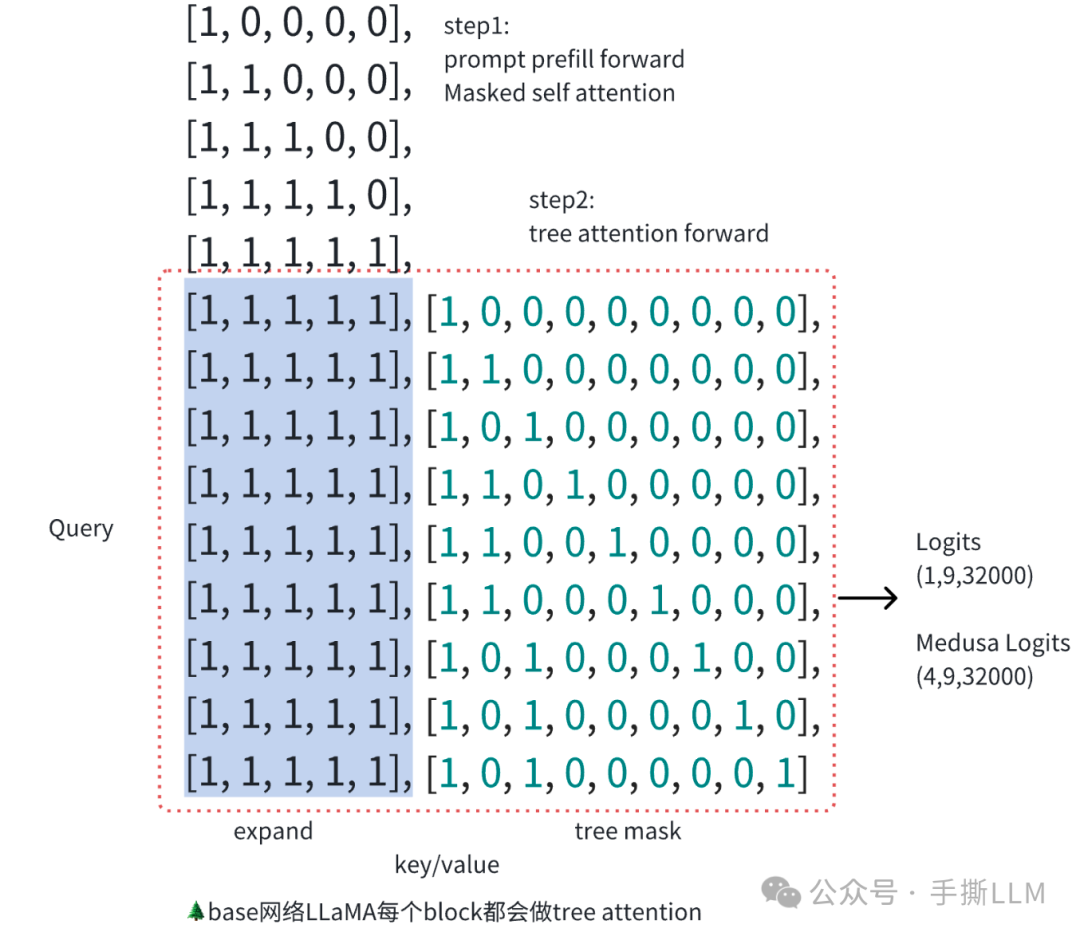
3.4.1 tree_decoding 实现细节

在Tree Decoding中，可见对Medusa做一次Forward，仅得到各路径logits, 不生成token

这里的model是Medusa
先计算一次LLaMA forward
再计算一次Medusa Head 输出

# medusa/model/utils.py   def tree_decoding(       model,       tree_candidates,       past_key_values,       medusa_position_ids,       input_ids,       retrieve_indices,   ):     	# 位置编码做一次shift，并非常规的       # normal: 1， 2， 3， 4， 5， |  6， 7， 8, 9, 10 11, 12, 13, 14       # shift :                      0,  1,  1, 2, 2, 2,  2,  2,  2       # pos   : 1， 2， 3， 4， 5， |  6,  7, 7, 8,  8, 8,  8, 8,  8     	position_ids = medusa_position_ids + input_ids.shape[1]              tree_medusa_logits, outputs, tree_logits = model(           tree_candidates,           output_orig=True,           past_key_values=past_key_values,           position_ids=position_ids,           medusa_forward=True,       )       logits = tree_logits[0, retrieve_indices]       medusa_logits = tree_medusa_logits[:, 0, retrieve_indices]       return medusa_logits, logits, outputs

实际上Tree Attention Machine 作用在 LLM 模型的Attention的计算中，事实上在3.4中的第二步骤，已经把 medusa_buffers["medusa_attn_mask"] 已经嵌入, 计算过程需要考虑past key value

outputs = self.base_model.model(       input_ids=input_ids,       attention_mask=attention_mask,       past_key_values=past_key_values,       position_ids=position_ids,   )   if output_orig:       orig = self.base_model.lm_head(outputs[0])

这里仅得到forward logits，无实际解码动作

3.4.2 计算最优路径

当前设定多个路径，在evaluate_posterior 计算出最优路径,

with torch.inference_mode():       medusa_logits, logits, outputs = tree_decoding(                   model,                   tree_candidates,                   past_key_values,                   medusa_buffers["medusa_position_ids"],                   input_ids,                   medusa_buffers["retrieve_indices"],               )              # reordering logits       # 原logits存放不连续，通过这两部复原成候选路径logits       logits = tree_logits[0, medusa_buffers["retrieve_indices"]       medusa_logits = tree_medusa_logits[:, 0, medusa_buffers["retrieve_indices"]              best_candidate, accept_length = evaluate_posterior(                   logits, candidates, temperature = 0, posterior_threshold = 0, posterior_alpha = 0               )       print('Medusa logits shape', medusa_logits.shape)       print('Logits shape', logits.shape)       print('Best candidate path index:', best_candidate.item())       print('Accept length:', accept_length.item())          print('Retrieved input @ best candidate:', tokenizer.batch_decode(candidates[best_candidate.item()]))   print('Retrieved output @ best candidate:', tokenizer.batch_decode(logits.argmax(-1)[best_candidate.item()]))      print('Retrieved input @ another candidate:', tokenizer.batch_decode(candidates[0]))   print('Retrieved output @ another candidate:', tokenizer.batch_decode(logits.argmax(-1)[0]))

输出结果为

Medusa logits shape torch.Size([4, 42, 5, 32000]) #4个头, 42条候选路径, 上一轮预测的Preds长度5，词表大小32000   Logits shape torch.Size([42, 5, 32000])   Best candidate path index: 14   Accept length: 3      Retrieved input @ best candidate: ['Once', 'upon', 'a', 'time', '<unk>']   Retrieved output @ best candidate: ['upon', 'a', 'time', ',', 'char']   Retrieved input @ another candidate: ['Once', 'upon', 'ly', 'time', 'a']   Retrieved output @ another candidate: ['upon', 'a', 'a', ',', 'char']

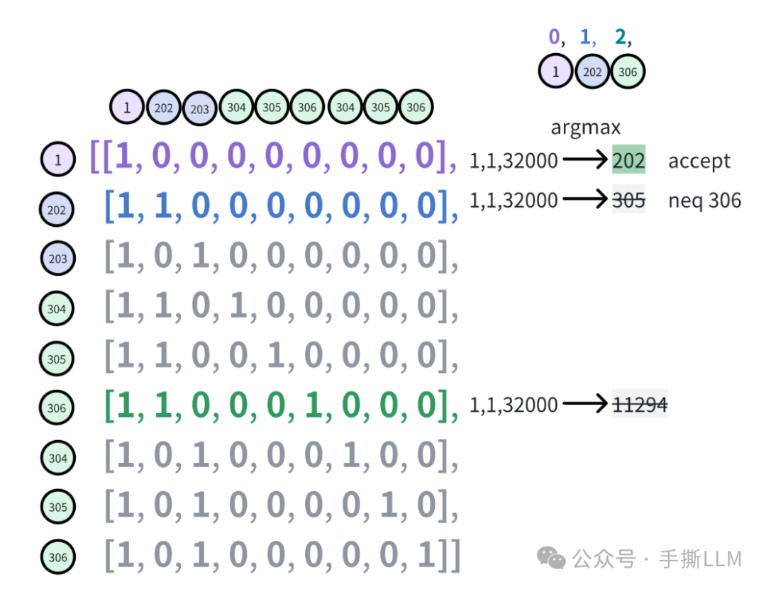
以下由于设定的温度参数是temperature=0, 依照baseline Greedy方式验证，得到最大路径

def evaluate_posterior(       logits, candidates, temperature, posterior_threshold=0.3, posterior_alpha = 0.09, top_p=0.8, sampling = 'typical', fast = True   ):       # Greedy decoding based on temperature value       if temperature == 0:            # Find the tokens that match the maximum logits for each position in the sequence           posterior_mask = (               candidates[:, 1:] == torch.argmax(logits[:, :-1], dim=-1)           ).int()           candidates_accept_length = (torch.cumprod(posterior_mask, dim=1)).sum(dim=1)           accept_length = candidates_accept_length.max()           # Choose the best candidate           if accept_length == 0:               # Default to the first candidate if none are accepted               best_candidate = torch.tensor(0, dtype=torch.long, device=candidates.device)           else:               best_candidate = torch.argmax(candidates_accept_length).to(torch.long)           return best_candidate, accept_length

简易表示一条路径的logits 及 agrmax取值, 对应代码实现为

原本logits矩阵如下，

			 `# reordering logits           logits = tree_logits[0, medusa_buffers["retrieve_indices"]           medusa_logits = tree_medusa_logits[:, 0, medusa_buffers["retrieve_indices"]          # [B,L,V] -> [Candidate_count, tree_depth, V]`

这种方式很简单check出accept length，但无法比较出同等长度解码路径的优劣出来。

3.5 小结

在这里我们解析了tree attention实现细节，相较第二章节baseline，我们基于稀疏树数据结构可以高效的在Top-10 中减少树搜索路径。

Tree Attention加入前后的接受率

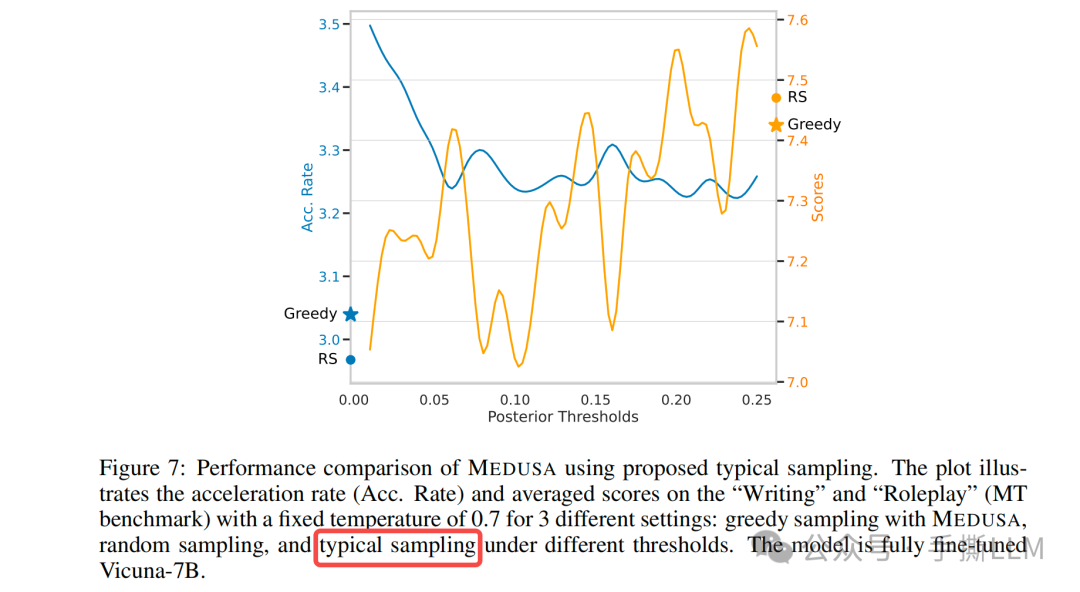
4 Typical Acceptance

在Medusa论文里采用了Typical Acceptance 解码策略，这种解码策略主要ref Typical Decoding 和 Truncation Sampling.

在Transformers库也支持这两种解码方式：

https://huggingface.co/docs/transformers/v4.38.2/en/main_classes/text_generation#transformers.GenerationConfig

GenerationConfig   	: typical_p        # for Typical Sampling   	: epsilon_cutoff   # for Trunction Sampling   	: eta_cutoff			 # for Trunction Sampling

使用Typical Acceptance解码策略后的接受率效果

4.1 原文评论

先看下原文对Speculative Decoding 的评价

随着温度增加，解码效率会急剧下降
尽管Draft model的分布对齐的很，但输出的结构任有概率被拒接掉

In speculative decoding papers [Leviathan et al., 2022, Chen et al., 2023], authors employ rejection sampling to yield diverse outputs that align with the distribution of the original model. However, subsequent implementations [Joao Gante, 2023, Spector and Re, 2023] reveal that this sampling strategy results in diminished efficiency as the sampling temperature increases. Intuitively, this can be comprehended in the extreme instance where the draft model is the same as the original one. Here, when using greedy decoding, all output of the draft model will be accepted, therefore maximizing the efficiency. Conversely, rejection sampling introduces extra overhead, as the draft model and the original model are sampled independently. Even if their distributions align perfectly, the output of the draft model may still be rejected.

在现实场景里，LLM通常被用来生成丰富的回答，用温度可以使得回答更有创造性，但是会导致输出分布不同，使得类似Speculative Sampling接受率低，Mudusa使用Typical Acceptance来提供接受率

However, in real-world scenarios, sampling from language models is often employed to generate diverse responses, and the temperature parameter is used merely to modulate the “creativity” of the response. Therefore, higher temperatures should result in more opportunities for the original model to accept the draft model’s output. We ascertain that it is typically unnecessary to match the distri bution of the original model. Thus, we propose employing a typical acceptance scheme to select plausible candidates rather than using rejection sampling. This approach draws inspiration from truncation sampling studies [Hewitt et al., 2022] (refer to Section 2 for an in-depth explanation). Our objective is to choose candidates that are typical, meaning they are not exceedingly improbable to be produced by the original model.

4.2 Typical Decoding 算法原理

Locally Typical Sampling

Typical Decoding 典型解码是一种基于信息的采样方法。

直观理解是我们在LLM解码过程，不需要太能predictable的词，也不能有太surprising的词，这样就能保证我们能得到丰富且避免重复生成的词汇

predictable：指的是条件概率下，生成的token可能性过大，一个例子是Donald 词后大概率会预测出Trump
surprising：指的是sampling出不同寻常的词，导致生成的质量差，比如跟着小冬瓜学习大模 采样出特

简要算法流程

假设token于此任务中，词汇表中的每个词预测的条件概率为

每个词汇条件熵为计算公式如下:

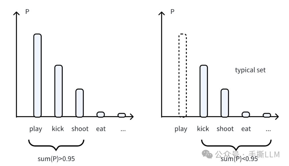
基于条件熵(top-p按概率)按增序重排候选序列，由后往前数累加概率和<0.95，如下图

满足条件的token归入到Typical set，再进行sampling解码，这样就能避免才到过于Predictable的词汇了。

此时typical set为

import torch   torch.set_printoptions(precision=4)      a = torch.tensor([0.15, 0.2, 0.30, 0.35])  # amazing   b = torch.tensor([0.01, 0.09, 0.2, 0.7]) # normal   c = torch.tensor([0.0001, 0.0049, 0.005, 0.99]) # predictable      def typical_metric(a, p):       print('p:', p)       print('token prob:', a)       entropy = -torch.sum(a * torch.log(a))       print("Entropy:", entropy)       sum = 0.0       sum_list = []       typical_set = []       condi_ents = []       for i in a:           condi_ent = entropy + torch.log(i)           condi_ents.append(condi_ent)           sum = sum + i.float()           sum_list.append(sum)           if sum<p:               typical_set.append(1)           else:               typical_set.append(0)       print(f'condi_entropy:',condi_ents)       print(f'typical sum:',sum_list)       print(f'typical set:',typical_set)       print('entrop dependent:',torch.exp(-entropy))       print('-'*50)          typical_metric(a, 0.5)   typical_metric(a, 0.95)   typical_metric(b, 0.95)   typical_metric(c, 0.95)

输出为

p: 0.5   token prob: tensor([0.1500, 0.2000, 0.3000, 0.3500])   Entropy: tensor(1.3351)   condi_entropy:   [tensor(-0.5620), tensor(-0.2744), tensor(0.1311), tensor(0.2853)]   typical sum:   [tensor(0.1500), tensor(0.3500), tensor(0.6500), tensor(1.)]   typical set:   [1, 1, 0, 0]   entrop dependent: tensor(0.2631)   --------------------------------------------------   p: 0.95   token prob: tensor([0.1500, 0.2000, 0.3000, 0.3500])   Entropy: tensor(1.3351)   condi_entropy:   [tensor(-0.5620), tensor(-0.2744), tensor(0.1311), tensor(0.2853)]   typical sum:   [tensor(0.1500), tensor(0.3500), tensor(0.6500), tensor(1.)]   typical set:   [1, 1, 1, 0]   entrop dependent: tensor(0.2631)   --------------------------------------------------   p: 0.95   token prob: tensor([0.0100, 0.0900, 0.2000, 0.7000])   Entropy: tensor(0.8343)   condi_entropy:   [tensor(-3.7708), tensor(-1.5736), tensor(-0.7751), tensor(0.4777)]   typical sum:   [tensor(0.0100), tensor(0.1000), tensor(0.3000), tensor(1.)]   typical set:   [1, 1, 1, 0]   entrop dependent: tensor(0.4342)   --------------------------------------------------   p: 0.95   token prob: tensor([1.0000e-04, 4.9000e-03, 5.0000e-03, 9.9000e-01])   Entropy: tensor(0.0634)   condi_entropy:   [tensor(-9.1469), tensor(-5.2551), tensor(-5.2349), tensor(0.0534)]   typical sum:   [tensor(1.0000e-04), tensor(0.0050), tensor(0.0100), tensor(1.)]   typical set:   [1, 1, 1, 0]   entrop dependent: tensor(0.9385)   --------------------------------------------------

4.3 Truction Sampling 算法原理

Truncation Sampling as Language Model Desmoothing

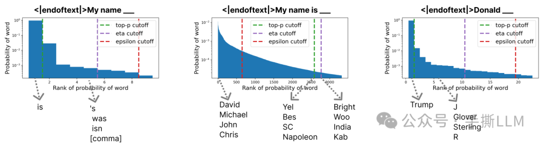
在Typical Sampling基础上，对概率低的token分布做一次截断，有两种策略

一种是 , 将概率低于阈值的token筛除掉

另一种 , 依赖一个固定阈值和条件熵的阈值来自适应的决定保留哪些token

选用不同的cut-off 策略，可以得到更加丰富的生成，最右侧图 Donald 在 eta cutoff中不会单一的采样到Trump

4.4 手撕Typical Acceptance

在理解Truction Sampling基础上，Medusa 通过比较目标预测的概率与traction sampling 阈值来确认是否接受

实现代码为

# ref: medusa/model/utils.py   # function evaluate_posterior()   import torch      logits = torch.randn(2,4,10) # 2个候选集合, 深度为4, vocab size为10   temperature = 1.5   posterior_threshold=0.3   posterior_alpha = 0.09   top_p=0.8,   candidates = [[0,0,0,1],[0,0,1,2]   candidates = torch.tensor(candidates)      # 开始计算信息   posterior_prob = torch.softmax(logits[:, :-1] / temperature, dim=-1)   print(posterior_prob.shape)   candidates_prob = torch.gather(       posterior_prob, dim=-1, index=candidates[:, 1:].unsqueeze(-1)   ).squeeze(-1)   posterior_entropy = -torch.sum(       posterior_prob * torch.log(posterior_prob + 1e-5), dim=-1   )    threshold = torch.minimum(       torch.ones_like(posterior_entropy) * posterior_threshold,       torch.exp(-posterior_entropy) * posterior_alpha,   )   print(candidates_prob)   print(threshold)   posterior_mask = candidates_prob > threshold   print(candidates_prob)   print(threshold)      # 计算接受的token   candidates_accept_length = (torch.cumprod(posterior_mask, dim=1)).sum(dim=1)   print(candidates_accept_length)      # 获取接受最长的token序列编号   accept_length = candidates_accept_length.max()   print('accept_length:', accept_length)      if accept_length == 0:       best_candidate = torch.tensor(0, dtype=torch.long, device=candidates.device)   else:       # 有多个候选集同样长度，取likelihood最大的序列作为best candidates       best_candidates = torch.where(candidates_accept_length == accept_length)[0]       likelihood = torch.sum(           torch.log(candidates_prob[best_candidates, :accept_length]), dim=-1       )       print(likelihood)       best_candidate = best_candidates[torch.argmax(likelihood)]   print(best_candidate)

输出为

torch.Size([2, 3, 10])   tensor([[0.0368, 0.0184, 0.0954],           [0.1382, 0.0433, 0.0704])   tensor([[0.0115, 0.0123, 0.0099],           [0.0106, 0.0130, 0.0099])   tensor([[0.0368, 0.0184, 0.0954],           [0.1382, 0.0433, 0.0704])   tensor([[0.0115, 0.0123, 0.0099],           [0.0106, 0.0130, 0.0099])   tensor([3, 3])   accept_length: tensor(3)   tensor([-9.6470, -7.7732])   tensor(1)

5. Medusa-2 训练

5.1 Medusa 训练策略

为了进一步提高Medusa head 的预测效率，Medusa-2采用联合训练的方式，有三种策略

Combined loss: 在训练Medusa-1时，同时加入backbone模型也进行参数训练，即增加next-token预测的loss
Differential learning rates: 由于backbone model已经充分训练了，而medusa需要更充分的训练，设定不同的learning rate可以达到目的
Head Warmup：

one-stage：先训练base model作为medusa-1，使用较少的epochs

two-stage：参照1的方式，进行混合训练，这里提到的warmup指逐步增大

在paper中描述

Besides this simple strategy, we can also use a more sophisticated warmup strategy by gradually increasing the weight _λ_0 of the backbone model’s loss. We find both strategies work well in practice

5.2 Self-Distillation

仅靠SFT训练，Medusa头只能适应给定的数据集的分布

那么这里可以采用self-distillation的方式使得Medusa头适应base model的分布

数据由base model以ShareGPT数据集作为种子进行Self-talk , 得到大量的backbone模型的输出作为蒸馏的Soft-label

For example, the model owners may only release the model without the training data, or the model may have gone through a Reinforcement Learning with Human Feedback (RLHF) procedure, which makes the output distribution of the model different from the training dataset. To tackle this issue, we propose an automated self-distillation pipeline to use the model itself to generate the training dataset for MEDUSA heads, which matches the output distribution of the model.

6. 总结

Medusa 是一种one-model 的并行解码框架, 采用多解码头、top-k候选+稀疏树、Typical Acceptantce和joint training+self distillation多种技巧来提高并行效率
Medusa 为了能达到更高的接受率采用的typical acceptance基于阈值方式解码，与原来的decoding分布不一致，精度期望进一步更多的实验体现，目前来看不同的训练策略有较大的差异，如Medusa 1和2加速比 2.18 -> 2.83
并行解码可以追溯到Transformer作者Noam Shazeer在18年提出的Blockwise Parallel Decoding, Medusa对该算法的继承和发扬，增加了很多新意和工程实现细节,

Reference

方佳瑞:LLM推理加速之Medusa：Blockwise Parallel Decoding的继承与发展
方佳瑞:LLM推理加速的文艺复兴：Noam Shazeer和Blockwise Parallel Decoding
Medusa
Speculative Decoidng
Blockwise parallel decoding
Typical Sampling
Truncation sampling
huggingface generation

如何系统的去学习大模型LLM ？

作为一名热心肠的互联网老兵，我意识到有很多经验和知识值得分享给大家，也可以通过我们的能力和经验解答大家在人工智能学习中的很多困惑，所以在工作繁忙的情况下还是坚持各种整理和分享。

但苦于知识传播途径有限，很多互联网行业朋友无法获得正确的资料得到学习提升，故此将并将重要的 AI大模型资料 包括AI大模型入门学习思维导图、精品AI大模型学习书籍手册、视频教程、实战学习等录播视频免费分享出来。

😝有需要的小伙伴，可以V扫描下方二维码免费领取🆓

在这里插入图片描述

一、全套AGI大模型学习路线

AI大模型时代的学习之旅：从基础到前沿，掌握人工智能的核心技能！

二、640套AI大模型报告合集

这套包含640份报告的合集，涵盖了AI大模型的理论研究、技术实现、行业应用等多个方面。无论您是科研人员、工程师，还是对AI大模型感兴趣的爱好者，这套报告合集都将为您提供宝贵的信息和启示。

三、AI大模型经典PDF籍

随着人工智能技术的飞速发展，AI大模型已经成为了当今科技领域的一大热点。这些大型预训练模型，如GPT-3、BERT、XLNet等，以其强大的语言理解和生成能力，正在改变我们对人工智能的认识。那以下这些PDF籍就是非常不错的学习资源。

在这里插入图片描述

四、AI大模型商业化落地方案

阶段1：AI大模型时代的基础理解

目标：了解AI大模型的基本概念、发展历程和核心原理。
内容：
- L1.1 人工智能简述与大模型起源
- L1.2 大模型与通用人工智能
- L1.3 GPT模型的发展历程
- L1.4 模型工程
  - L1.4.1 知识大模型
  - L1.4.2 生产大模型
  - L1.4.3 模型工程方法论
  - L1.4.4 模型工程实践
- L1.5 GPT应用案例

阶段2：AI大模型API应用开发工程

目标：掌握AI大模型API的使用和开发，以及相关的编程技能。
内容：
- L2.1 API接口
  - L2.1.1 OpenAI API接口
  - L2.1.2 Python接口接入
  - L2.1.3 BOT工具类框架
  - L2.1.4 代码示例
- L2.2 Prompt框架
  - L2.2.1 什么是Prompt
  - L2.2.2 Prompt框架应用现状
  - L2.2.3 基于GPTAS的Prompt框架
  - L2.2.4 Prompt框架与Thought
  - L2.2.5 Prompt框架与提示词
- L2.3 流水线工程
  - L2.3.1 流水线工程的概念
  - L2.3.2 流水线工程的优点
  - L2.3.3 流水线工程的应用
- L2.4 总结与展望

阶段3：AI大模型应用架构实践

目标：深入理解AI大模型的应用架构，并能够进行私有化部署。
内容：
- L3.1 Agent模型框架
  - L3.1.1 Agent模型框架的设计理念
  - L3.1.2 Agent模型框架的核心组件
  - L3.1.3 Agent模型框架的实现细节
- L3.2 MetaGPT
  - L3.2.1 MetaGPT的基本概念
  - L3.2.2 MetaGPT的工作原理
  - L3.2.3 MetaGPT的应用场景
- L3.3 ChatGLM
  - L3.3.1 ChatGLM的特点
  - L3.3.2 ChatGLM的开发环境
  - L3.3.3 ChatGLM的使用示例
- L3.4 LLAMA
  - L3.4.1 LLAMA的特点
  - L3.4.2 LLAMA的开发环境
  - L3.4.3 LLAMA的使用示例
- L3.5 其他大模型介绍