mindspore打卡第24天之LSTM+CRF序列标注

LSTM+CRF序列标注

  

概述

序列标注指给定输入序列，给序列中每个Token进行标注标签的过程。序列标注问题通常用于从文本中进行信息抽取，包括分词(Word Segmentation)、词性标注(Position Tagging)、命名实体识别(Named Entity Recognition, NER)等。以命名实体识别为例：

输入序列	清	华	大	学	座	落	于	首	都	北	京
输出标注	B	I	I	I	O	O	O	O	O	B	I

如上表所示，清华大学 和 北京是地名，需要将其识别，我们对每个输入的单词预测其标签，最后根据标签来识别实体。

这里使用了一种常见的命名实体识别的标注方法——“BIOE”标注，将一个实体(Entity)的开头标注为B，其他部分标注为I，非实体标注为O。

条件随机场(Conditional Random Field, CRF)

从上文的举例可以看到，对序列进行标注，实际上是对序列中每个Token进行标签预测，可以直接视作简单的多分类问题。但是序列标注不仅仅需要对单个Token进行分类预测，同时相邻Token直接有关联关系。以清华大学一词为例:

输入序列	清	华	大	学
输出标注	B	I	I	I	√
输出标注	O	I	I	I	×

如上表所示，正确的实体中包含的4个Token有依赖关系，I前必须是B或I，而错误输出结果将清字标注为O，违背了这一依赖。将命名实体识别视为多分类问题，则每个词的预测概率都是独立的，易产生类似的问题，因此需要引入一种能够学习到此种关联关系的算法来保证预测结果的正确性。而条件随机场是适合此类场景的一种概率图模型。下面对条件随机场的定义和参数化形式进行简析。

考虑到序列标注问题的线性序列特点，本节所述的条件随机场特指线性链条件随机场(Linear Chain CRF)

设 x = { x 0 , . . . , x n } x=\{x_0, ..., x_n\} x={x0​,...,xn​}为输入序列， y = { y 0 , . . . , y n } ， y ∈ Y y=\{y_0, ..., y_n\}，y \in Y y={y0​,...,yn​}，y∈Y为输出的标注序列，其中$n$为序列的最大长度，$Y$表示$x$对应的所有可能的输出序列集合。则输出序列$y$的概率为：

$$\begin{array}{r}P(y|x)=\frac{\exp (\text{Score}(x,y))}{{\sum }_{y^{\prime }\in Y}\exp (\text{Score}(x,y^{\prime }))}(1)\end{array}$$

设$x_i$, $y_i$为序列的第$i$个Token和对应的标签，则$\text{Score}$需要能够在计算$x_i$和$y_i$的映射的同时，捕获相邻标签$y_{i-1}$和$y_i$之间的关系，因此我们定义两个概率函数：

1. 发射概率函数${\psi }_{\text{EMIT}}$：表示$x_i\to y_i$的概率。
2. 转移概率函数${\psi }_{\text{TRANS}}$：表示$y_{i-1}\to y_i$的概率。

则可以得到$\text{Score}$的计算公式：

$$\begin{array}{r}\text{Score}(x,y)=\sum _i\log {\psi }_{\text{EMIT}}(x_i\to y_i)+\log {\psi }_{\text{TRANS}}(y_{i-1}\to y_i)(2)\end{array}$$

设标签集合为$T$，构造大小为$|T|x|T|$的矩阵$\text{P}$，用于存储标签间的转移概率；由编码层(可以为Dense、LSTM等)输出的隐状态$h$可以直接视作发射概率，此时$\text{Score}$的计算公式可以转化为：

$$\begin{array}{r}\text{Score}(x,y)=\sum _i{h}_i[y_i]+{\text{P}}_{y_{i-1},y_i}(3)\end{array}$$

条件随机场（Conditional Random Field, CRF）是一种用于建模序列数据的统计建模方法，特别适用于序列标注和分类问题，如命名实体识别（NER）、词性标注（POS tagging）等。CRF能够捕捉序列中标签之间的依赖关系，这是它相比于其他序列标注模型的一个显著优势。下面我们将深入解析CRF在序列标注问题中的工作原理。

CRF的定义和参数化

对于一个输入序列 x = { x 0 , . . . , x n } x=\{x_0,...,x_n\} x={x0​,...,xn​}和其对应的输出序列（或标签序列） y = { y 0 , . . . , y n } y=\{y_0,...,y_n\} y={y0​,...,yn​}，其中$y\in Y$，$Y$是所有可能的输出序列集合，CRF的目标是学习一个条件概率分布$P(y|x)$，这个分布表示在给定输入序列$x$的情况下输出序列$y$的概率。

Score函数

在CRF中，我们定义一个Score函数来衡量一个特定的输出序列$y$对于给定输入序列$x$的可能性。Score函数通常由两部分组成：

1. 发射分数：${\psi }_{\text{EMIT}}(x_i\to y_i)$，表示输入序列中位置$i$的元素$x_i$被标注为标签$y_i$的概率。
2. 转移分数：${\psi }_{\text{TRANS}}(y_{i-1}\to y_i)$，表示从标签$y_{i-1}$转移到标签$y_i$的概率。

Score函数是这两部分的加权和：

$$\text{Score}(x,y)=\sum _i{\psi }_{\text{EMIT}}(x_i\to y_i)+{\psi }_{\text{TRANS}}(y_{i-1}\to y_i)$$

在实际应用中，为了方便数学运算，通常会取对数，这样乘法就变成了加法：

$$\text{Score}(x,y)=\sum _i\log {\psi }_{\text{EMIT}}(x_i\to y_i)+\log {\psi }_{\text{TRANS}}(y_{i-1}\to y_i)$$

归一化

由于Score函数只衡量了序列的可能性，但没有归一化成概率，因此我们需要通过Z(x)即归一化因子来实现概率分布的归一化：

$$P(y|x)=\frac{\exp (\text{Score}(x,y))}{{\sum }_{y^{\prime }\in Y}\exp (\text{Score}(x,y^{\prime }))}$$

这里的分母${\sum }_{y^{\prime }\in Y}\exp (\text{Score}(x,y^{\prime }))$被称为分区函数（partition function），它确保了$P(y|x)$是一个有效的概率分布，即所有可能的$y$的$P(y|x)$之和等于1。

参数化Score函数

在现代深度学习框架中，Score函数的参数化通常更加灵活。例如，发射分数可以是神经网络（如Dense层或LSTM层）的输出，而转移分数则可以通过一个转移矩阵$\mathbf{P}$来表示，其中${\mathbf{P}}_{y_{i-1},y_i}$表示从标签$y_{i-1}$转移到$y_i$的分数。

最终，Score函数可以写作：

$$\text{Score}(x,y)=\sum _i{h}_i[y_i]+{\mathbf{P}}_{y_{i-1},y_i}$$

这里$h_i$是神经网络在位置$i$的输出，可以看作是$x_i$的发射分数的参数化表示。

小结

CRF通过显式地建模序列中标签之间的依赖关系，以及输入特征与标签之间的关系，提供了更准确的序列标注能力。在深度学习中，CRF常常作为最后一层，位于神经网络之上，以利用神经网络的强表达能力，同时保留CRF的全局最优属性，从而提高序列标注的准确性。

在条件随机场(CRF)的上下文中，我们可以用一个具体的例子来说明输入和输出的计算过程。假设我们的任务是中文的命名实体识别(NER)，并且我们使用的是线性链CRF。我们将以一句话“李明在北京大学上学。”作为输入序列，目标是识别出其中的实体。

输入序列

输入序列是：“李明在北京大学上学。”，我们可以将其分解为一系列的字符或者词汇，取决于我们的输入表示方式。在这里，我们假设使用字符级的表示，所以输入序列变为：

x = ["李", "明", "在", "北", "京", "大", "学", "上", "学", "。"]

输出序列

输出序列是一系列的实体标签，假设我们使用BIO标注格式（Begin, Inside, Outside），则正确的输出序列应该是：

y = ["B-PER", "I-PER", "O", "B-ORG", "I-ORG", "I-ORG", "I-ORG", "O", "O", "O"]

计算过程

现在，我们来具体看一下如何使用CRF计算某个输出序列$y$的条件概率$P(y|x)$。

Step 1: 定义Score函数

Score函数$\text{Score}(x,y)$包含了两部分：发射分数和转移分数。

• 发射分数：对于每个位置$i$，发射分数${\psi }_{\text{EMIT}}(x_i\to y_i)$表示在位置$i$处，字符$x_i$被标记为$y_i$的概率。在神经网络模型中，这通常是通过一个全连接层加上softmax函数来实现的，给出每个位置上所有可能标签的概率分布。

• 转移分数：转移分数${\psi }_{\text{TRANS}}(y_{i-1}\to y_i)$表示从标签$y_{i-1}$转移到标签$y_i$的概率。在CRF中，这通常通过一个转移矩阵$\mathbf{P}$来实现，其中${\mathbf{P}}_{y_{i-1},y_i}$表示从$y_{i-1}$转移到$y_i$的分数。

Step 2: 计算Score函数

对于输入序列$x$和输出序列$y$，Score函数可以写作：
$$\text{Score}(x,y)=\sum _i{h}_i[y_i]+{\mathbf{P}}_{y_{i-1},y_i}$$

其中$h_i[y_i]$是从神经网络得到的发射分数，${\mathbf{P}}_{y_{i-1},y_i}$是从转移矩阵$\mathbf{P}$中查找到的转移分数。

Step 3: 归一化

最后，我们需要将Score函数归一化为条件概率$P(y|x)$。这涉及到计算所有可能输出序列的Score函数的指数和，也就是分区函数$Z(x)$：
$$Z(x)=\sum _{y^{\prime }\in Y}\exp (\text{Score}(x,y^{\prime }))$$

然后，$P(y|x)$可以写作：
$$P(y|x)=\frac{\exp (\text{Score}(x,y))}{Z(x)}$$

示例计算

假设在某个时刻，我们正在计算位置$i=3$处的Score，即字符“北”。假设它的发射分数$h_3["B-ORG"]=0.8$，而转移分数${\mathbf{P}}_{y_2,y_3}={\mathbf{P}}_{O,B-ORG}=0.7$（假设前一个标签是“O”，即“在”的标签）。那么在位置$i=3$处的贡献为：
$${\text{Score}}_i=h_3["B-ORG"]+{\mathbf{P}}_{O,B-ORG}=0.8+0.7=1.5$$

最终，整个序列的Score将是所有位置$i$处的Score之和，然后通过归一化得到条件概率$P(y|x)$。

请注意，实际的Score函数计算会涉及指数和对数操作，以避免数值稳定性和效率问题，但上述过程给出了基本的计算框架。

完整的CRF完整推导可参考Log-Linear Models, MEMMs, and CRFs

接下来我们根据上述公式，使用MindSpore来实现CRF的参数化形式。首先实现CRF层的前向训练部分，将CRF和损失函数做合并，选择分类问题常用的负对数似然函数(Negative Log Likelihood, NLL)，则有：

$$\begin{array}{r}\text{Loss}=-log(P(y|x))(4)\end{array}$$

由公式$(1)$可得，

$$\begin{array}{r}\text{Loss}=-log(\frac{\exp (\text{Score}(x,y))}{{\sum }_{y^{\prime }\in Y}\exp (\text{Score}(x,y^{\prime }))})(5)\end{array}$$

$$\begin{array}{r}=log(\sum _{y^{\prime }\in Y}\exp (\text{Score}(x,y^{\prime }))-\text{Score}(x,y)\end{array}$$

根据公式$(5)$，我们称被减数为Normalizer，减数为Score，分别实现后相减得到最终Loss。

Score计算

首先根据公式$(3)$计算正确标签序列所对应的得分，这里需要注意，除了转移概率矩阵$\text{P}$外，还需要维护两个大小为$|T|$的向量，分别作为序列开始和结束时的转移概率。同时我们引入了一个掩码矩阵$mask$，将多个序列打包为一个Batch时填充的值忽略，使得$\text{Score}$计算仅包含有效的Token。

在计算Score的过程中，我们确实需要考虑到一些额外的细节，比如序列的起始和终止，以及在处理不同长度的序列时如何有效利用掩码矩阵（mask）来排除填充部分的影响。下面我将详细介绍如何在CRF中进行这样的Score计算。

起始和终止转移概率

在CRF中，我们通常会添加一个虚拟的起始状态和一个虚拟的终止状态。这样做的目的是为了完整地描述整个序列的状态转移过程。在转移矩阵$\mathbf{P}$中，我们会加入从起始状态到第一个标签的转移概率，以及从最后一个标签到终止状态的转移概率。

设$S$为起始状态，$E$为终止状态，那么$\mathbf{P}$的大小实际上是$(|T|+2)\times (|T|+2)$，其中$|T|$是除去起始和终止状态的实际标签集合的大小。${\mathbf{P}}_{S,y_0}$表示从起始状态到序列第一个标签$y_0$的转移概率，而${\mathbf{P}}_{y_n,E}$表示从序列最后一个标签$y_n$到终止状态的转移概率。

掩码矩阵的作用

在处理Batch中的多个序列时，由于序列长度不同，较短的序列会被填充至与最长序列相同长度。掩码矩阵$mask$是用来标记哪些位置是真实数据，哪些位置是填充的。$mask$通常是一个二进制矩阵，其中1表示该位置是真实数据，0表示该位置是填充的。

在计算Score时，$mask$可以帮助我们跳过填充部分，只计算有意义的Token。具体来说，$mask$可以与发射分数和转移分数相乘，这样填充部分的贡献就被置为了0，不会影响最终的Score。

具体计算过程

对于一个Batch中的序列，我们按照以下步骤计算Score：

1. 初始化Score为0。
2. 对于每个序列中的每个位置$i$：
   • 计算发射分数$h_i[y_i]$，其中$y_i$是位置$i$的标签。
   • 如果$i>0$，计算转移分数${\mathbf{P}}_{y_{i-1},y_i}$。
   • 将发射分数和转移分数相加，并乘以$mask[i]$，这样填充部分的分数会被忽略。
   • 将得到的结果累加到当前的Score上。
3. 对于序列的起始和终止，分别加上起始转移分数${\mathbf{P}}_{S,y_0}$和终止转移分数${\mathbf{P}}_{y_n,E}$。
4. 最终得到的Score就是该序列在给定标签下的总分。

这个过程确保了Score的计算既考虑了序列内部的标签依赖关系，也处理了不同长度序列的批量计算问题。通过掩码矩阵的应用，我们可以有效地避免填充部分的干扰，使得计算过程更加精确和高效。

%%capture captured_output
# 实验环境已经预装了mindspore==2.2.14，如需更换mindspore版本，可更改下面mindspore的版本号
!pip uninstall mindspore -y
!pip install -i https://pypi.mirrors.ustc.edu.cn/simple mindspore==2.2.14

# 查看当前 mindspore 版本
!pip show mindspore

Name: mindspore
Version: 2.2.14
Summary: MindSpore is a new open source deep learning training/inference framework that could be used for mobile, edge and cloud scenarios.
Home-page: https://www.mindspore.cn
Author: The MindSpore Authors
Author-email: contact@mindspore.cn
License: Apache 2.0
Location: /home/nginx/miniconda/envs/jupyter/lib/python3.9/site-packages
Requires: asttokens, astunparse, numpy, packaging, pillow, protobuf, psutil, scipy
Required-by: 

def compute_score(emissions, tags, seq_ends, mask, trans, start_trans, end_trans):
    # emissions: (seq_length, batch_size, num_tags)
    # tags: (seq_length, batch_size)
    # mask: (seq_length, batch_size)

    seq_length, batch_size = tags.shape
    mask = mask.astype(emissions.dtype)

    # 将score设置为初始转移概率
    # shape: (batch_size,)
    score = start_trans[tags[0]]
    # score += 第一次发射概率
    # shape: (batch_size,)
    score += emissions[0, mnp.arange(batch_size), tags[0]]

    for i in range(1, seq_length):
        # 标签由i-1转移至i的转移概率（当mask == 1时有效）
        # shape: (batch_size,)
        score += trans[tags[i - 1], tags[i]] * mask[i]

        # 预测tags[i]的发射概率（当mask == 1时有效）
        # shape: (batch_size,)
        score += emissions[i, mnp.arange(batch_size), tags[i]] * mask[i]

    # 结束转移
    # shape: (batch_size,)
    last_tags = tags[seq_ends, mnp.arange(batch_size)]
    # score += 结束转移概率
    # shape: (batch_size,)
    score += end_trans[last_tags]

    return score

Normalizer计算

根据公式$(5)$，Normalizer是$x$对应的所有可能的输出序列的Score的对数指数和(Log-Sum-Exp)。此时如果按穷举法进行计算，则需要将每个可能的输出序列Score都计算一遍，共有$|T{|}^n$个结果。这里我们采用动态规划算法，通过复用计算结果来提高效率。

假设需要计算从第$0$至第$i$个Token所有可能的输出序列得分${\text{Score}}_i$，则可以先计算出从第$0$至第$i-1$个Token所有可能的输出序列得分${\text{Score}}_{i-1}$。因此，Normalizer可以改写为以下形式：

$$log(\sum _{y_{0,i}^{\prime }\in Y}\exp ({\text{Score}}_i))=log(\sum _{y_{0,i-1}^{\prime }\in Y}\exp ({\text{Score}}_{i-1}+h_i+\text{P}))(6)$$

其中$h_i$为第$i$个Token的发射概率，$\text{P}$是转移矩阵。由于发射概率矩阵$h$和转移概率矩阵$\text{P}$独立于$y$的序列路径计算，可以将其提出，可得：

$$log(\sum _{y_{0,i}^{\prime }\in Y}\exp ({\text{Score}}_i))=log(\sum _{y_{0,i-1}^{\prime }\in Y}\exp ({\text{Score}}_{i-1}))+h_i+\text{P}(7)$$

根据公式(7)，Normalizer的实现如下：

Normalizer的计算是CRF中一个关键步骤，它用于计算所有可能的输出序列的Score的对数指数和，即Log-Sum-Exp（LSE）操作，以保证最终的条件概率分布是规范化的。在计算Normalizer时，我们采用动态规划算法，避免了直接枚举所有可能序列的高计算成本，从而提高了计算效率。

动态规划算法

在动态规划中，我们递归地计算每个位置$i$上所有可能标签的累积分数，直到序列的末尾。这个累积分数表示从序列开始到当前位置$i$，经过所有可能的标签序列路径的Log-Sum-Exp分数。

1. 初始化：对于序列的第一个Token，我们计算从起始状态到每个可能标签的Score。这相当于计算起始转移分数加上第一个Token的发射分数，得到一个大小为$|T|$的向量。

2. 递推：对于每个后续的位置$i$，我们计算从所有可能的前一个位置的标签到当前位置标签的Score。这涉及到两个步骤：

   • 计算前一个位置的累积分数${\text{Score}}_{i-1}$加上当前位置的发射分数$h_i$和转移矩阵$\mathbf{P}$。
   • 进行Log-Sum-Exp操作，合并所有前一个位置到当前位置的路径分数，得到一个新的大小为$|T|$的向量，代表当前位置所有可能标签的累积分数。

3. 终止：到达序列的最后一个Token时，我们计算从最后一个Token的每个可能标签到终止状态的Score，得到最终的Normalizer。

具体实现

具体到公式(7)，我们看到动态规划的关键在于复用先前计算的结果，即${\text{Score}}_{i-1}$，来计算${\text{Score}}_i$。但是，我们不能直接将$h_i$和$\mathbf{P}$提出，因为它们与路径选择相关。正确的做法是先计算所有可能的前一个标签到当前标签的转移分数，再进行Log-Sum-Exp操作。

对于每个位置$i$，动态规划的更新规则可以写为：
$${\alpha }_i(y_i)=\log \left(\sum _{y_{i-1}\in T}\exp \left({\alpha }_{i-1}(y_{i-1})+{\mathbf{P}}_{y_{i-1},y_i}+h_i[y_i]\right)\right)$$

其中，${\alpha }_i(y_i)$表示到达位置$i$，标签为$y_i$的累积Log-Sum-Exp分数。最终的Normalizer就是序列最后一个位置所有可能标签的${\alpha }_i(y_i)$的Log-Sum-Exp。

通过这种方式，我们只需要线性时间复杂度$O(n|T{|}^2)$就能计算出Normalizer，大大减少了计算量，使得CRF在大规模序列标注任务中成为可行的解决方案。

def compute_normalizer(emissions, mask, trans, start_trans, end_trans):
    # emissions: (seq_length, batch_size, num_tags)
    # mask: (seq_length, batch_size)

    seq_length = emissions.shape[0]

    # 将score设置为初始转移概率，并加上第一次发射概率
    # shape: (batch_size, num_tags)
    score = start_trans + emissions[0]

    for i in range(1, seq_length):
        # 扩展score的维度用于总score的计算
        # shape: (batch_size, num_tags, 1)
        broadcast_score = score.expand_dims(2)

        # 扩展emission的维度用于总score的计算
        # shape: (batch_size, 1, num_tags)
        broadcast_emissions = emissions[i].expand_dims(1)

        # 根据公式(7)，计算score_i
        # 此时broadcast_score是由第0个到当前Token所有可能路径
        # 对应score的log_sum_exp
        # shape: (batch_size, num_tags, num_tags)
        next_score = broadcast_score + trans + broadcast_emissions

        # 对score_i做log_sum_exp运算，用于下一个Token的score计算
        # shape: (batch_size, num_tags)
        next_score = ops.logsumexp(next_score, axis=1)

        # 当mask == 1时，score才会变化
        # shape: (batch_size, num_tags)
        score = mnp.where(mask[i].expand_dims(1), next_score, score)

    # 最后加结束转移概率
    # shape: (batch_size, num_tags)
    score += end_trans
    # 对所有可能的路径得分求log_sum_exp
    # shape: (batch_size,)
    return ops.logsumexp(score, axis=1)

Viterbi算法

在完成前向训练部分后，需要实现解码部分。这里我们选择适合求解序列最优路径的Viterbi算法。与计算Normalizer类似，使用动态规划求解所有可能的预测序列得分。不同的是在解码时同时需要将第$i$个Token对应的score取值最大的标签保存，供后续使用Viterbi算法求解最优预测序列使用。

取得最大概率得分$\text{Score}$，以及每个Token对应的标签历史$\text{History}$后，根据Viterbi算法可以得到公式：

$$P_{0,i}=max(P_{0,i-1})+P_{i-1,i}$$

从第0个至第$i$个Token对应概率最大的序列，只需要考虑从第0个至第$i-1$个Token对应概率最大的序列，以及从第$i$个至第$i-1$个概率最大的标签即可。因此我们逆序求解每一个概率最大的标签，构成最佳的预测序列。

由于静态图语法限制，我们将Viterbi算法求解最佳预测序列的部分作为后处理函数，不纳入后续CRF层的实现。

Viterbi Algorithm for Decoding

在CRF模型的解码阶段，我们利用Viterbi算法来找到最有可能的标签序列，即具有最高概率的序列路径。与正向训练阶段计算所有可能序列的归一化概率不同，Viterbi算法专注于寻找单个最优序列。动态规划是实现Viterbi算法的核心技术，它通过递归地构建每个位置的最佳路径来找到全局最优解。

算法步骤

1. 初始化：与Normalizer计算一样，我们从序列的第一个Token开始，计算从起始状态到每个可能标签的Score，这构成了动态规划表格的第一列。

2. 递归构建：对于每个后续位置$i$，我们计算到达每个可能标签$y_i$的最佳路径Score。这涉及到：

   • 查找前一个位置$i-1$上的每个可能标签$y_{i-1}$，以及从$y_{i-1}$到$y_i$的转移分数${\mathbf{P}}_{y_{i-1},y_i}$。
   • 添加当前位置的发射分数$h_i[y_i]$。
   • 从所有可能的前一个标签中选取使得路径Score最大的那个标签，记为${\text{BestPrevTag}}_{i-1}$。

   因此，到达位置$i$的每个标签$y_i$的最佳路径Score可以表示为：
   $${\text{BestPathScore}}_i(y_i)=\underset{y_{i-1}\in T}{\max }({\text{BestPathScore}}_{i-1}(y_{i-1})+{\mathbf{P}}_{y_{i-1},y_i}+h_i[y_i])$$

   并且记录下使上述表达式取最大值的前一个标签${\text{BestPrevTag}}_{i-1}$。

3. 回溯：在到达序列的最后一个Token时，我们得到了每个可能标签的最佳路径Score。我们选取这些Score中的最大值，以及对应的标签，作为序列的最后一个标签。然后，我们逆序回溯，根据之前记录的$\text{BestPrevTag}$来重建整个最优标签序列。

解码过程

在实际操作中，Viterbi算法的解码部分通常是在模型的推理阶段进行的，作为模型预测的一部分。由于Viterbi算法涉及的动态规划表格和回溯步骤，它通常被设计为一个单独的后处理函数，不直接包含在模型的前向传播计算图中。这是因为动态规划表格的构建和回溯步骤可能不适合某些深度学习框架的自动梯度计算机制，尤其是在静态图模式下。

实现细节

在实现Viterbi算法时，我们需要注意以下几点：

• 动态规划表格：用于存储每个位置每个标签的最佳路径Score，以及指向其前一个最佳标签的指针。
• 边界处理：起始和终止状态的处理，确保算法正确地开始和结束。
• 数值稳定性：在计算路径Score时，使用对数概率和Log-Sum-Exp操作来避免数值溢出或下溢问题。

通过Viterbi算法，我们可以在CRF模型中高效地解码出最优的标签序列，即使在面对复杂的序列标注任务时，也能保持较高的准确性和效率。

def viterbi_decode(emissions, mask, trans, start_trans, end_trans):
    # emissions: (seq_length, batch_size, num_tags)
    # mask: (seq_length, batch_size)

    seq_length = mask.shape[0]

    score = start_trans + emissions[0]
    history = ()

    for i in range(1, seq_length):
        broadcast_score = score.expand_dims(2)
        broadcast_emission = emissions[i].expand_dims(1)
        next_score = broadcast_score + trans + broadcast_emission

        # 求当前Token对应score取值最大的标签，并保存
        indices = next_score.argmax(axis=1)
        history += (indices,)

        next_score = next_score.max(axis=1)
        score = mnp.where(mask[i].expand_dims(1), next_score, score)

    score += end_trans

    return score, history

def post_decode(score, history, seq_length):
    # 使用Score和History计算最佳预测序列
    batch_size = seq_length.shape[0]
    seq_ends = seq_length - 1
    # shape: (batch_size,)
    best_tags_list = []

    # 依次对一个Batch中每个样例进行解码
    for idx in range(batch_size):
        # 查找使最后一个Token对应的预测概率最大的标签，
        # 并将其添加至最佳预测序列存储的列表中
        best_last_tag = score[idx].argmax(axis=0)
        best_tags = [int(best_last_tag.asnumpy())]

        # 重复查找每个Token对应的预测概率最大的标签，加入列表
        for hist in reversed(history[:seq_ends[idx]]):
            best_last_tag = hist[idx][best_tags[-1]]
            best_tags.append(int(best_last_tag.asnumpy()))

        # 将逆序求解的序列标签重置为正序
        best_tags.reverse()
        best_tags_list.append(best_tags)

    return best_tags_list

CRF层

完成上述前向训练和解码部分的代码后，将其组装完整的CRF层。考虑到输入序列可能存在Padding的情况，CRF的输入需要考虑输入序列的真实长度，因此除发射矩阵和标签外，加入seq_length参数传入序列Padding前的长度，并实现生成mask矩阵的sequence_mask方法。

综合上述代码，使用nn.Cell进行封装，最后实现完整的CRF层如下：

import mindspore as ms
import mindspore.nn as nn
import mindspore.ops as ops
import mindspore.numpy as mnp
from mindspore.common.initializer import initializer, Uniform

def sequence_mask(seq_length, max_length, batch_first=False):
    """根据序列实际长度和最大长度生成mask矩阵"""
    range_vector = mnp.arange(0, max_length, 1, seq_length.dtype)
    result = range_vector < seq_length.view(seq_length.shape + (1,))
    if batch_first:
        return result.astype(ms.int64)
    return result.astype(ms.int64).swapaxes(0, 1)

class CRF(nn.Cell):
    def __init__(self, num_tags: int, batch_first: bool = False, reduction: str = 'sum') -> None:
        if num_tags <= 0:
            raise ValueError(f'invalid number of tags: {num_tags}')
        super().__init__()
        if reduction not in ('none', 'sum', 'mean', 'token_mean'):
            raise ValueError(f'invalid reduction: {reduction}')
        self.num_tags = num_tags
        self.batch_first = batch_first
        self.reduction = reduction
        self.start_transitions = ms.Parameter(initializer(Uniform(0.1), (num_tags,)), name='start_transitions')
        self.end_transitions = ms.Parameter(initializer(Uniform(0.1), (num_tags,)), name='end_transitions')
        self.transitions = ms.Parameter(initializer(Uniform(0.1), (num_tags, num_tags)), name='transitions')

    def construct(self, emissions, tags=None, seq_length=None):
        if tags is None:
            return self._decode(emissions, seq_length)
        return self._forward(emissions, tags, seq_length)

    def _forward(self, emissions, tags=None, seq_length=None):
        if self.batch_first:
            batch_size, max_length = tags.shape
            emissions = emissions.swapaxes(0, 1)
            tags = tags.swapaxes(0, 1)
        else:
            max_length, batch_size = tags.shape

        if seq_length is None:
            seq_length = mnp.full((batch_size,), max_length, ms.int64)

        mask = sequence_mask(seq_length, max_length)

        # shape: (batch_size,)
        numerator = compute_score(emissions, tags, seq_length-1, mask, self.transitions, self.start_transitions, self.end_transitions)
        # shape: (batch_size,)
        denominator = compute_normalizer(emissions, mask, self.transitions, self.start_transitions, self.end_transitions)
        # shape: (batch_size,)
        llh = denominator - numerator

        if self.reduction == 'none':
            return llh
        if self.reduction == 'sum':
            return llh.sum()
        if self.reduction == 'mean':
            return llh.mean()
        return llh.sum() / mask.astype(emissions.dtype).sum()

    def _decode(self, emissions, seq_length=None):
        if self.batch_first:
            batch_size, max_length = emissions.shape[:2]
            emissions = emissions.swapaxes(0, 1)
        else:
            batch_size, max_length = emissions.shape[:2]

        if seq_length is None:
            seq_length = mnp.full((batch_size,), max_length, ms.int64)

        mask = sequence_mask(seq_length, max_length)

        return viterbi_decode(emissions, mask, self.transitions, self.start_transitions, self.end_transitions)

BiLSTM+CRF模型

在实现CRF后，我们设计一个双向LSTM+CRF的模型来进行命名实体识别任务的训练。模型结构如下：

nn.Embedding -> nn.LSTM -> nn.Dense -> CRF

其中LSTM提取序列特征，经过Dense层变换获得发射概率矩阵，最后送入CRF层。具体实现如下：

class BiLSTM_CRF(nn.Cell):
    def __init__(self, vocab_size, embedding_dim, hidden_dim, num_tags, padding_idx=0):
        super().__init__()
        self.embedding = nn.Embedding(vocab_size, embedding_dim, padding_idx=padding_idx)
        self.lstm = nn.LSTM(embedding_dim, hidden_dim // 2, bidirectional=True, batch_first=True)
        self.hidden2tag = nn.Dense(hidden_dim, num_tags, 'he_uniform')
        self.crf = CRF(num_tags, batch_first=True)

    def construct(self, inputs, seq_length, tags=None):
        embeds = self.embedding(inputs)
        outputs, _ = self.lstm(embeds, seq_length=seq_length)
        feats = self.hidden2tag(outputs)

        crf_outs = self.crf(feats, tags, seq_length)
        return crf_outs

完成模型设计后，我们生成两句例子和对应的标签，并构造词表和标签表。

embedding_dim = 16
hidden_dim = 32

training_data = [(
    "清 华 大 学 坐 落 于 首 都 北 京".split(),
    "B I I I O O O O O B I".split()
), (
    "重 庆 是 一 个 魔 幻 城 市".split(),
    "B I O O O O O O O".split()
)]

word_to_idx = {}
word_to_idx['<pad>'] = 0
for sentence, tags in training_data:
    for word in sentence:
        if word not in word_to_idx:
            word_to_idx[word] = len(word_to_idx)

tag_to_idx = {"B": 0, "I": 1, "O": 2}

len(word_to_idx)

21

接下来实例化模型，选择优化器并将模型和优化器送入Wrapper。

由于CRF层已经进行了NLLLoss的计算，因此不需要再设置Loss。

model = BiLSTM_CRF(len(word_to_idx), embedding_dim, hidden_dim, len(tag_to_idx))
optimizer = nn.SGD(model.trainable_params(), learning_rate=0.01, weight_decay=1e-4)

grad_fn = ms.value_and_grad(model, None, optimizer.parameters)

def train_step(data, seq_length, label):
    loss, grads = grad_fn(data, seq_length, label)
    optimizer(grads)
    return loss

将生成的数据打包成Batch，按照序列最大长度，对长度不足的序列进行填充，分别返回输入序列、输出标签和序列长度构成的Tensor。

def prepare_sequence(seqs, word_to_idx, tag_to_idx):
    seq_outputs, label_outputs, seq_length = [], [], []
    max_len = max([len(i[0]) for i in seqs])

    for seq, tag in seqs:
        seq_length.append(len(seq))
        idxs = [word_to_idx[w] for w in seq]
        labels = [tag_to_idx[t] for t in tag]
        idxs.extend([word_to_idx['<pad>'] for i in range(max_len - len(seq))])
        labels.extend([tag_to_idx['O'] for i in range(max_len - len(seq))])
        seq_outputs.append(idxs)
        label_outputs.append(labels)

    return ms.Tensor(seq_outputs, ms.int64), \
            ms.Tensor(label_outputs, ms.int64), \
            ms.Tensor(seq_length, ms.int64)

data, label, seq_length = prepare_sequence(training_data, word_to_idx, tag_to_idx)
data.shape, label.shape, seq_length.shape

((2, 11), (2, 11), (2,))

对模型进行预编译后，训练500个step。

训练流程可视化依赖tqdm库，可使用pip install tqdm命令安装。

from tqdm import tqdm

steps = 500
with tqdm(total=steps) as t:
    for i in range(steps):
        loss = train_step(data, seq_length, label)
        t.set_postfix(loss=loss)
        t.update(1)

  0%|          | 0/500 [00:00<?, ?it/s]

/

100%|██████████| 500/500 [04:14<00:00,  1.97it/s, loss=0.34322357] 

最后我们来观察训练500个step后的模型效果，首先使用模型预测可能的路径得分以及候选序列。

score, history = model(data, seq_length)
score

\




Tensor(shape=[2, 3], dtype=Float32, value=
[[ 3.03385792e+01,  3.49243088e+01,  2.98639412e+01],
 [ 2.74814892e+01,  2.51049538e+01,  3.22654572e+01]])

使用后处理函数进行预测得分的后处理。

predict = post_decode(score, history, seq_length)
predict

[[0, 1, 1, 1, 2, 2, 2, 2, 2, 0, 1], [0, 1, 2, 2, 2, 2, 2, 2, 2]]

最后将预测的index序列转换为标签序列，打印输出结果，查看效果。

idx_to_tag = {idx: tag for tag, idx in tag_to_idx.items()}

def sequence_to_tag(sequences, idx_to_tag):
    outputs = []
    for seq in sequences:
        outputs.append([idx_to_tag[i] for i in seq])
    return outputs

sequence_to_tag(predict, idx_to_tag)

[['B', 'I', 'I', 'I', 'O', 'O', 'O', 'O', 'O', 'B', 'I'],
 ['B', 'I', 'O', 'O', 'O', 'O', 'O', 'O', 'O']]

print("yangge  mindspore打卡第24天之LSTM+CRF序列标注 2023 07 12")

yangge  mindspore打卡第24天之LSTM+CRF序列标注 2023 07 12

RNN实现情感分类

  

概述

情感分类是自然语言处理中的经典任务，是典型的分类问题。本节使用MindSpore实现一个基于RNN网络的情感分类模型，实现如下的效果：

输入: This film is terrible
正确标签: Negative
预测标签: Negative

输入: This film is great
正确标签: Positive
预测标签: Positive

数据准备

本节使用情感分类的经典数据集IMDB影评数据集，数据集包含Positive和Negative两类，下面为其样例：

Review	Label
“Quitting” may be as much about exiting a pre-ordained identity as about drug withdrawal. As a rural guy coming to Beijing, class and success must have struck this young artist face on as an appeal to separate from his roots and far surpass his peasant parents’ acting success. Troubles arise, however, when the new man is too new, when it demands too big a departure from family, history, nature, and personal identity. The ensuing splits, and confusion between the imaginary and the real and the dissonance between the ordinary and the heroic are the stuff of a gut check on the one hand or a complete escape from self on the other.	Negative
This movie is amazing because the fact that the real people portray themselves and their real life experience and do such a good job it’s like they’re almost living the past over again. Jia Hongsheng plays himself an actor who quit everything except music and drugs struggling with depression and searching for the meaning of life while being angry at everyone especially the people who care for him most.	Positive

此外，需要使用预训练词向量对自然语言单词进行编码，以获取文本的语义特征，本节选取Glove词向量作为Embedding。

数据下载模块

为了方便数据集和预训练词向量的下载，首先设计数据下载模块，实现可视化下载流程，并保存至指定路径。数据下载模块使用requests库进行http请求，并通过tqdm库对下载百分比进行可视化。此外针对下载安全性，使用IO的方式下载临时文件，而后保存至指定的路径并返回。

tqdm和requests库需手动安装，命令如下：pip install tqdm requests

%%capture captured_output
# 实验环境已经预装了mindspore==2.2.14，如需更换mindspore版本，可更改下面mindspore的版本号
!pip uninstall mindspore -y
!pip install -i https://pypi.mirrors.ustc.edu.cn/simple mindspore==2.2.14

# 查看当前 mindspore 版本
!pip show mindspore

Name: mindspore
Version: 2.2.14
Summary: MindSpore is a new open source deep learning training/inference framework that could be used for mobile, edge and cloud scenarios.
Home-page: https://www.mindspore.cn
Author: The MindSpore Authors
Author-email: contact@mindspore.cn
License: Apache 2.0
Location: /home/nginx/miniconda/envs/jupyter/lib/python3.9/site-packages
Requires: asttokens, astunparse, numpy, packaging, pillow, protobuf, psutil, scipy
Required-by: 

import os
import shutil
import requests
import tempfile
from tqdm import tqdm
from typing import IO
from pathlib import Path

# 指定保存路径为 `home_path/.mindspore_examples`
cache_dir = Path.home() / '.mindspore_examples'

def http_get(url: str, temp_file: IO):
    """使用requests库下载数据，并使用tqdm库进行流程可视化"""
    req = requests.get(url, stream=True)
    content_length = req.headers.get('Content-Length')
    total = int(content_length) if content_length is not None else None
    progress = tqdm(unit='B', total=total)
    for chunk in req.iter_content(chunk_size=1024):
        if chunk:
            progress.update(len(chunk))
            temp_file.write(chunk)
    progress.close()

def download(file_name: str, url: str):
    """下载数据并存为指定名称"""
    if not os.path.exists(cache_dir):
        os.makedirs(cache_dir)
    cache_path = os.path.join(cache_dir, file_name)
    cache_exist = os.path.exists(cache_path)
    if not cache_exist:
        with tempfile.NamedTemporaryFile() as temp_file:
            http_get(url, temp_file)
            temp_file.flush()
            temp_file.seek(0)
            with open(cache_path, 'wb') as cache_file:
                shutil.copyfileobj(temp_file, cache_file)
    return cache_path

完成数据下载模块后，下载IMDB数据集进行测试(此处使用华为云的镜像用于提升下载速度)。下载过程及保存的路径如下：

imdb_path = download('aclImdb_v1.tar.gz', 'https://mindspore-website.obs.myhuaweicloud.com/notebook/datasets/aclImdb_v1.tar.gz')
imdb_path

'/home/nginx/.mindspore_examples/aclImdb_v1.tar.gz'

加载IMDB数据集

下载好的IMDB数据集为tar.gz文件，我们使用Python的tarfile库对其进行读取，并将所有数据和标签分别进行存放。原始的IMDB数据集解压目录如下：

    ├── aclImdb
    │   ├── imdbEr.txt
    │   ├── imdb.vocab
    │   ├── README
    │   ├── test
    │   └── train
    │         ├── neg
    │         ├── pos
    ...

数据集已分割为train和test两部分，且每部分包含neg和pos两个分类的文件夹，因此需分别train和test进行读取并处理数据和标签。

import re
import six
import string
import tarfile

class IMDBData():
    """IMDB数据集加载器

    加载IMDB数据集并处理为一个Python迭代对象。

    """
    label_map = {
        "pos": 1,
        "neg": 0
    }
    def __init__(self, path, mode="train"):
        self.mode = mode
        self.path = path
        self.docs, self.labels = [], []

        self._load("pos")
        self._load("neg")

    def _load(self, label):
        pattern = re.compile(r"aclImdb/{}/{}/.*\.txt$".format(self.mode, label))
        # 将数据加载至内存
        with tarfile.open(self.path) as tarf:
            tf = tarf.next()
            while tf is not None:
                if bool(pattern.match(tf.name)):
                    # 对文本进行分词、去除标点和特殊字符、小写处理
                    self.docs.append(str(tarf.extractfile(tf).read().rstrip(six.b("\n\r"))
                                         .translate(None, six.b(string.punctuation)).lower()).split())
                    self.labels.append([self.label_map[label]])
                tf = tarf.next()

    def __getitem__(self, idx):
        return self.docs[idx], self.labels[idx]

    def __len__(self):
        return len(self.docs)

完成IMDB数据加载器后，加载训练数据集进行测试，输出数据集数量：

imdb_train = IMDBData(imdb_path, 'train')
len(imdb_train)

25000

将IMDB数据集加载至内存并构造为迭代对象后，可以使用mindspore.dataset提供的Generatordataset接口加载数据集迭代对象，并进行下一步的数据处理，下面封装一个函数将train和test分别使用Generatordataset进行加载，并指定数据集中文本和标签的column_name分别为text和label:

import mindspore.dataset as ds

def load_imdb(imdb_path):
    imdb_train = ds.GeneratorDataset(IMDBData(imdb_path, "train"), column_names=["text", "label"], shuffle=True, num_samples=10000)
    imdb_test = ds.GeneratorDataset(IMDBData(imdb_path, "test"), column_names=["text", "label"], shuffle=False)
    return imdb_train, imdb_test

加载IMDB数据集，可以看到imdb_train是一个GeneratorDataset对象。

imdb_train, imdb_test = load_imdb(imdb_path)
imdb_train

<mindspore.dataset.engine.datasets_user_defined.GeneratorDataset at 0xfffecef43dc0>

加载预训练词向量

预训练词向量是对输入单词的数值化表示，通过nn.Embedding层，采用查表的方式，输入单词对应词表中的index，获得对应的表达向量。
因此进行模型构造前，需要将Embedding层所需的词向量和词表进行构造。这里我们使用Glove(Global Vectors for Word Representation)这种经典的预训练词向量，
其数据格式如下：

Word	Vector
the	0.418 0.24968 -0.41242 0.1217 0.34527 -0.044457 -0.49688 -0.17862 -0.00066023 …
,	0.013441 0.23682 -0.16899 0.40951 0.63812 0.47709 -0.42852 -0.55641 -0.364 …

我们直接使用第一列的单词作为词表，使用dataset.text.Vocab将其按顺序加载；同时读取每一行的Vector并转为numpy.array，用于nn.Embedding加载权重使用。具体实现如下：

import zipfile
import numpy as np

def load_glove(glove_path):
    glove_100d_path = os.path.join(cache_dir, 'glove.6B.100d.txt')
    if not os.path.exists(glove_100d_path):
        glove_zip = zipfile.ZipFile(glove_path)
        glove_zip.extractall(cache_dir)

    embeddings = []
    tokens = []
    with open(glove_100d_path, encoding='utf-8') as gf:
        for glove in gf:
            word, embedding = glove.split(maxsplit=1)
            tokens.append(word)
            embeddings.append(np.fromstring(embedding, dtype=np.float32, sep=' '))
    # 添加 <unk>, <pad> 两个特殊占位符对应的embedding
    embeddings.append(np.random.rand(100))
    embeddings.append(np.zeros((100,), np.float32))

    vocab = ds.text.Vocab.from_list(tokens, special_tokens=["<unk>", "<pad>"], special_first=False)
    embeddings = np.array(embeddings).astype(np.float32)
    return vocab, embeddings

由于数据集中可能存在词表没有覆盖的单词，因此需要加入<unk>标记符；同时由于输入长度的不一致，在打包为一个batch时需要将短的文本进行填充，因此需要加入<pad>标记符。完成后的词表长度为原词表长度+2。

下面下载Glove词向量，并加载生成词表和词向量权重矩阵。

glove_path = download('glove.6B.zip', 'https://mindspore-website.obs.myhuaweicloud.com/notebook/datasets/glove.6B.zip')
vocab, embeddings = load_glove(glove_path)
len(vocab.vocab())

400002

使用词表将the转换为index id，并查询词向量矩阵对应的词向量：

idx = vocab.tokens_to_ids('the')
embedding = embeddings[idx]
idx, embedding

(0,
 array([-0.038194, -0.24487 ,  0.72812 , -0.39961 ,  0.083172,  0.043953,
        -0.39141 ,  0.3344  , -0.57545 ,  0.087459,  0.28787 , -0.06731 ,
         0.30906 , -0.26384 , -0.13231 , -0.20757 ,  0.33395 , -0.33848 ,
        -0.31743 , -0.48336 ,  0.1464  , -0.37304 ,  0.34577 ,  0.052041,
         0.44946 , -0.46971 ,  0.02628 , -0.54155 , -0.15518 , -0.14107 ,
        -0.039722,  0.28277 ,  0.14393 ,  0.23464 , -0.31021 ,  0.086173,
         0.20397 ,  0.52624 ,  0.17164 , -0.082378, -0.71787 , -0.41531 ,
         0.20335 , -0.12763 ,  0.41367 ,  0.55187 ,  0.57908 , -0.33477 ,
        -0.36559 , -0.54857 , -0.062892,  0.26584 ,  0.30205 ,  0.99775 ,
        -0.80481 , -3.0243  ,  0.01254 , -0.36942 ,  2.2167  ,  0.72201 ,
        -0.24978 ,  0.92136 ,  0.034514,  0.46745 ,  1.1079  , -0.19358 ,
        -0.074575,  0.23353 , -0.052062, -0.22044 ,  0.057162, -0.15806 ,
        -0.30798 , -0.41625 ,  0.37972 ,  0.15006 , -0.53212 , -0.2055  ,
        -1.2526  ,  0.071624,  0.70565 ,  0.49744 , -0.42063 ,  0.26148 ,
        -1.538   , -0.30223 , -0.073438, -0.28312 ,  0.37104 , -0.25217 ,
         0.016215, -0.017099, -0.38984 ,  0.87424 , -0.72569 , -0.51058 ,
        -0.52028 , -0.1459  ,  0.8278  ,  0.27062 ], dtype=float32))

数据集预处理

通过加载器加载的IMDB数据集进行了分词处理，但不满足构造训练数据的需要，因此要对其进行额外的预处理。其中包含的预处理如下：

• 通过Vocab将所有的Token处理为index id。
• 将文本序列统一长度，不足的使用<pad>补齐，超出的进行截断。

这里我们使用mindspore.dataset中提供的接口进行预处理操作。这里使用到的接口均为MindSpore的高性能数据引擎设计，每个接口对应操作视作数据流水线的一部分，详情请参考MindSpore数据引擎。
首先针对token到index id的查表操作，使用text.Lookup接口，将前文构造的词表加载，并指定unknown_token。其次为文本序列统一长度操作，使用PadEnd接口，此接口定义最大长度和补齐值(pad_value)，这里我们取最大长度为500，填充值对应词表中<pad>的index id。

除了对数据集中text进行预处理外，由于后续模型训练的需要，要将label数据转为float32格式。

import mindspore as ms

lookup_op = ds.text.Lookup(vocab, unknown_token='<unk>')
pad_op = ds.transforms.PadEnd([500], pad_value=vocab.tokens_to_ids('<pad>'))
type_cast_op = ds.transforms.TypeCast(ms.float32)

完成预处理操作后，需将其加入到数据集处理流水线中，使用map接口对指定的column添加操作。

imdb_train = imdb_train.map(operations=[lookup_op, pad_op], input_columns=['text'])
imdb_train = imdb_train.map(operations=[type_cast_op], input_columns=['label'])

imdb_test = imdb_test.map(operations=[lookup_op, pad_op], input_columns=['text'])
imdb_test = imdb_test.map(operations=[type_cast_op], input_columns=['label'])

由于IMDB数据集本身不包含验证集，我们手动将其分割为训练和验证两部分，比例取0.7, 0.3。

imdb_train, imdb_valid = imdb_train.split([0.7, 0.3])

[WARNING] ME(6421:281473410185520,MainProcess):2024-07-12-04:47:08.954.566 [mindspore/dataset/engine/datasets.py:1203] Dataset is shuffled before split.

最后指定数据集的batch大小，通过batch接口指定，并设置是否丢弃无法被batch size整除的剩余数据。

调用数据集的map、split、batch为数据集处理流水线增加对应操作，返回值为新的Dataset类型。现在仅定义流水线操作，在执行时开始执行数据处理流水线，获取最终处理好的数据并送入模型进行训练。

imdb_train = imdb_train.batch(64, drop_remainder=True)
imdb_valid = imdb_valid.batch(64, drop_remainder=True)

模型构建

完成数据集的处理后，我们设计用于情感分类的模型结构。首先需要将输入文本(即序列化后的index id列表)通过查表转为向量化表示，此时需要使用nn.Embedding层加载Glove词向量；然后使用RNN循环神经网络做特征提取；最后将RNN连接至一个全连接层，即nn.Dense，将特征转化为与分类数量相同的size，用于后续进行模型优化训练。整体模型结构如下：

nn.Embedding -> nn.RNN -> nn.Dense

这里我们使用能够一定程度规避RNN梯度消失问题的变种LSTM(Long short-term memory)做特征提取层。下面对模型进行详解：

Embedding

Embedding层又可称为EmbeddingLookup层，其作用是使用index id对权重矩阵对应id的向量进行查找，当输入为一个由index id组成的序列时，则查找并返回一个相同长度的矩阵，例如：

embedding = nn.Embedding(1000, 100) # 词表大小(index的取值范围)为1000，表示向量的size为100
input shape: (1, 16)                # 序列长度为16
output shape: (1, 16, 100)

这里我们使用前文处理好的Glove词向量矩阵，设置nn.Embedding的embedding_table为预训练词向量矩阵。对应的vocab_size为词表大小400002，embedding_size为选用的glove.6B.100d向量大小，即100。

RNN(循环神经网络)

循环神经网络（Recurrent Neural Network, RNN）是一类以序列（sequence）数据为输入，在序列的演进方向进行递归（recursion）且所有节点（循环单元）按链式连接的神经网络。下图为RNN的一般结构：

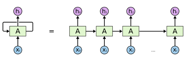
图示左侧为一个RNN Cell循环，右侧为RNN的链式连接平铺。实际上不管是单个RNN Cell还是一个RNN网络，都只有一个Cell的参数，在不断进行循环计算中更新。

由于RNN的循环特性，和自然语言文本的序列特性(句子是由单词组成的序列)十分匹配，因此被大量应用于自然语言处理研究中。下图为RNN的结构拆解：

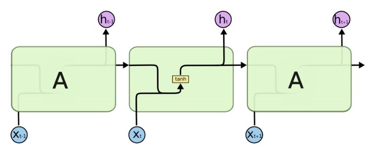
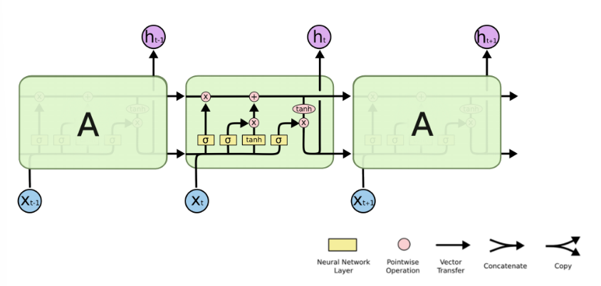
RNN单个Cell的结构简单，因此也造成了梯度消失(Gradient Vanishing)问题，具体表现为RNN网络在序列较长时，在序列尾部已经基本丢失了序列首部的信息。为了克服这一问题，LSTM(Long short-term memory)被提出，通过门控机制(Gating Mechanism)来控制信息流在每个循环步中的留存和丢弃。下图为LSTM的结构拆解：

本节我们选择LSTM变种而不是经典的RNN做特征提取，来规避梯度消失问题，并获得更好的模型效果。下面来看MindSpore中nn.LSTM对应的公式：

$$h_{0:t},(h_t,c_t)=\text{LSTM}(x_{0:t},(h_0,c_0))$$

这里nn.LSTM隐藏了整个循环神经网络在序列时间步(Time step)上的循环，送入输入序列、初始状态，即可获得每个时间步的隐状态(hidden state)拼接而成的矩阵，以及最后一个时间步对应的隐状态。我们使用最后的一个时间步的隐状态作为输入句子的编码特征，送入下一层。

Time step：在循环神经网络计算的每一次循环，成为一个Time step。在送入文本序列时，一个Time step对应一个单词。因此在本例中，LSTM的输出$h_{0:t}$对应每个单词的隐状态集合，$h_t$和$c_t$对应最后一个单词对应的隐状态。

Dense

在经过LSTM编码获取句子特征后，将其送入一个全连接层，即nn.Dense，将特征维度变换为二分类所需的维度1，经过Dense层后的输出即为模型预测结果。

import math
import mindspore as ms
import mindspore.nn as nn
import mindspore.ops as ops
from mindspore.common.initializer import Uniform, HeUniform

class RNN(nn.Cell):
    def __init__(self, embeddings, hidden_dim, output_dim, n_layers,
                 bidirectional, pad_idx):
        super().__init__()
        vocab_size, embedding_dim = embeddings.shape
        self.embedding = nn.Embedding(vocab_size, embedding_dim, embedding_table=ms.Tensor(embeddings), padding_idx=pad_idx)
        self.rnn = nn.LSTM(embedding_dim,
                           hidden_dim,
                           num_layers=n_layers,
                           bidirectional=bidirectional,
                           batch_first=True)
        weight_init = HeUniform(math.sqrt(5))
        bias_init = Uniform(1 / math.sqrt(hidden_dim * 2))
        self.fc = nn.Dense(hidden_dim * 2, output_dim, weight_init=weight_init, bias_init=bias_init)

    def construct(self, inputs):
        embedded = self.embedding(inputs)
        _, (hidden, _) = self.rnn(embedded)
        hidden = ops.concat((hidden[-2, :, :], hidden[-1, :, :]), axis=1)
        output = self.fc(hidden)
        return output

损失函数与优化器

完成模型主体构建后，首先根据指定的参数实例化网络；然后选择损失函数和优化器。针对本节情感分类问题的特性，即预测Positive或Negative的二分类问题，我们选择nn.BCEWithLogitsLoss(二分类交叉熵损失函数)。

hidden_size = 256
output_size = 1
num_layers = 2
bidirectional = True
lr = 0.001
pad_idx = vocab.tokens_to_ids('<pad>')

model = RNN(embeddings, hidden_size, output_size, num_layers, bidirectional, pad_idx)
loss_fn = nn.BCEWithLogitsLoss(reduction='mean')
optimizer = nn.Adam(model.trainable_params(), learning_rate=lr)

训练逻辑

在完成模型构建，进行训练逻辑的设计。一般训练逻辑分为一下步骤：

1. 读取一个Batch的数据；
2. 送入网络，进行正向计算和反向传播，更新权重；
3. 返回loss。

下面按照此逻辑，使用tqdm库，设计训练一个epoch的函数，用于训练过程和loss的可视化。

def forward_fn(data, label):
    logits = model(data)
    loss = loss_fn(logits, label)
    return loss

grad_fn = ms.value_and_grad(forward_fn, None, optimizer.parameters)

def train_step(data, label):
    loss, grads = grad_fn(data, label)
    optimizer(grads)
    return loss

def train_one_epoch(model, train_dataset, epoch=0):
    model.set_train()
    total = train_dataset.get_dataset_size()
    loss_total = 0
    step_total = 0
    with tqdm(total=total) as t:
        t.set_description('Epoch %i' % epoch)
        for i in train_dataset.create_tuple_iterator():
            loss = train_step(*i)
            loss_total += loss.asnumpy()
            step_total += 1
            t.set_postfix(loss=loss_total/step_total)
            t.update(1)

评估指标和逻辑

训练逻辑完成后，需要对模型进行评估。即使用模型的预测结果和测试集的正确标签进行对比，求出预测的准确率。由于IMDB的情感分类为二分类问题，对预测值直接进行四舍五入即可获得分类标签(0或1)，然后判断是否与正确标签相等即可。下面为二分类准确率计算函数实现：

def binary_accuracy(preds, y):
    """
    计算每个batch的准确率
    """

    # 对预测值进行四舍五入
    rounded_preds = np.around(ops.sigmoid(preds).asnumpy())
    correct = (rounded_preds == y).astype(np.float32)
    acc = correct.sum() / len(correct)
    return acc

有了准确率计算函数后，类似于训练逻辑，对评估逻辑进行设计, 分别为以下步骤：

1. 读取一个Batch的数据；
2. 送入网络，进行正向计算，获得预测结果；
3. 计算准确率。

同训练逻辑一样，使用tqdm进行loss和过程的可视化。此外返回评估loss至供保存模型时作为模型优劣的判断依据。

在进行evaluate时，使用的模型是不包含损失函数和优化器的网络主体；
在进行evaluate前，需要通过model.set_train(False)将模型置为评估状态，此时Dropout不生效。

def evaluate(model, test_dataset, criterion, epoch=0):
    total = test_dataset.get_dataset_size()
    epoch_loss = 0
    epoch_acc = 0
    step_total = 0
    model.set_train(False)

    with tqdm(total=total) as t:
        t.set_description('Epoch %i' % epoch)
        for i in test_dataset.create_tuple_iterator():
            predictions = model(i[0])
            loss = criterion(predictions, i[1])
            epoch_loss += loss.asnumpy()

            acc = binary_accuracy(predictions, i[1])
            epoch_acc += acc

            step_total += 1
            t.set_postfix(loss=epoch_loss/step_total, acc=epoch_acc/step_total)
            t.update(1)

    return epoch_loss / total

模型训练与保存

前序完成了模型构建和训练、评估逻辑的设计，下面进行模型训练。这里我们设置训练轮数为5轮。同时维护一个用于保存最优模型的变量best_valid_loss，根据每一轮评估的loss值，取loss值最小的轮次，将模型进行保存。为节省用例运行时长，此处num_epochs设置为2，可根据需要自行修改。

num_epochs = 2
best_valid_loss = float('inf')
ckpt_file_name = os.path.join(cache_dir, 'sentiment-analysis.ckpt')

for epoch in range(num_epochs):
    train_one_epoch(model, imdb_train, epoch)
    valid_loss = evaluate(model, imdb_valid, loss_fn, epoch)

    if valid_loss < best_valid_loss:
        best_valid_loss = valid_loss
        ms.save_checkpoint(model, ckpt_file_name)

Epoch 0:   0%|          | 0/109 [00:00<?, ?it/s]

|

Epoch 0: 100%|██████████| 109/109 [13:30<00:00,  7.44s/it, loss=0.688]  
Epoch 0: 100%|██████████| 46/46 [00:38<00:00,  1.18it/s, acc=0.593, loss=0.677]
Epoch 1: 100%|██████████| 109/109 [01:25<00:00,  1.27it/s, loss=0.683]
Epoch 1: 100%|██████████| 46/46 [00:13<00:00,  3.42it/s, acc=0.602, loss=0.671]

可以看到每轮Loss逐步下降，在验证集上的准确率逐步提升。

模型加载与测试

模型训练完成后，一般需要对模型进行测试或部署上线，此时需要加载已保存的最优模型(即checkpoint)，供后续测试使用。这里我们直接使用MindSpore提供的Checkpoint加载和网络权重加载接口：1.将保存的模型Checkpoint加载到内存中，2.将Checkpoint加载至模型。

load_param_into_net接口会返回模型中没有和Checkpoint匹配的权重名，正确匹配时返回空列表。

param_dict = ms.load_checkpoint(ckpt_file_name)
ms.load_param_into_net(model, param_dict)

([], [])

对测试集打batch，然后使用evaluate方法进行评估，得到模型在测试集上的效果。

imdb_test = imdb_test.batch(64)
evaluate(model, imdb_test, loss_fn)

Epoch 0: 100%|█████████▉| 390/391 [01:28<00:00,  4.54it/s, acc=0.58, loss=0.676] 

-

Epoch 0: 100%|██████████| 391/391 [03:06<00:00,  2.09it/s, acc=0.581, loss=0.676]





0.6757554032308671

自定义输入测试

最后我们设计一个预测函数，实现开头描述的效果，输入一句评价，获得评价的情感分类。具体包含以下步骤:

1. 将输入句子进行分词；
2. 使用词表获取对应的index id序列；
3. index id序列转为Tensor；
4. 送入模型获得预测结果；
5. 打印输出预测结果。

具体实现如下：

score_map = {
    1: "Positive",
    0: "Negative"
}

def predict_sentiment(model, vocab, sentence):
    model.set_train(False)
    tokenized = sentence.lower().split()
    indexed = vocab.tokens_to_ids(tokenized)
    tensor = ms.Tensor(indexed, ms.int32)
    tensor = tensor.expand_dims(0)
    prediction = model(tensor)
    return score_map[int(np.round(ops.sigmoid(prediction).asnumpy()))]

最后我们预测开头的样例，可以看到模型可以很好地将评价语句的情感进行分类。

predict_sentiment(model, vocab, "This film is terrible")

'Positive'

predict_sentiment(model, vocab, "This film is great")

'Positive'

print("yangge  mindspore打卡第24天之RNN实现情感分类 2023 07 12")

yangge  mindspore打卡第24天之RNN实现情感分类 2023 07 12