机器学习（五） -- 监督学习（7） --SVM2

系列文章目录及链接

上篇：机器学习（五） -- 监督学习（7） --SVM1
下篇：

前言

tips：标题前有“***”的内容为补充内容，是给好奇心重的宝宝看的，可自行跳过。文章内容被“文章内容”删除线标记的，也可以自行跳过。“！！！”一般需要特别注意或者容易出错的地方。

本系列文章是作者边学习边总结的，内容有不对的地方还请多多指正，同时本系列文章会不断完善，每篇文章不定时会有修改。

由于作者时间不算富裕，有些内容的《算法实现》部分暂未完善，以后有时间再来补充。见谅！

文中为方便理解，会将接口在用到的时候才导入，实际中应在文件开始统一导入。

 三、**算法实现

四、接口实现

1、API

sklearn.svm.SVC
 
导入：
from sklearn.svm import SVC
 
语法：
SVC(C=1.0, kernel=‘rbf’, degree=3, gamma=‘auto’,
coef0=0.0, shrinking=True, probability=False,tol=0.001,
cache_size=200, class_weight=None, verbose=False, max_iter=-1,
decision_function_shape=None,random_state=None)

    C：惩罚参数，默认值是1.0。
        C越大，表示越不允许分类出错，这样对训练集测试时准确率很高，但泛化能力弱。
        C值小，对误分类的惩罚减小，允许容错，将他们当成噪声点，泛化能力较强。
    Kernel：核函数，默认是rbf，
        ‘linear’：为线性核，C越大分类效果越好，但可能会过拟合；
        ‘rbf’：为高斯核，gamma值越小，分类界面越连续；gamma值越大，分类界面越“散”，分类效果越好，但可能会过拟合；
        ‘poly’：多项式核
        ‘sigmoid’：Sigmoid核函数 
        ‘precomputed’：核矩阵
    decision_function_shape ：‘ovo’, ‘ovr’ or None, default=None
        'ovr'时，为one v rest,即一个类别与其他ov类别进行划分；
        'ovo'时，为one v one,即将类别两两进行划分，用二分类的方法模拟多分类的结果；
    degree ：多项式poly函数的维度，默认是3，选择其他核函数时会被忽略。
    gamma ：‘rbf’,‘poly’ 和‘sigmoid’的核函数参数。默认是’auto’，则会选择1/n_features
    coef0 ：核函数的常数项。对于‘poly’和 ‘sigmoid’有用。
    probability ：是否采用概率估计？.默认为False
    shrinking ：是否采用shrinking heuristic方法，默认为true
    tol ：停止训练的误差值大小，默认为1e-3
    cache_size ：核函数cache缓存大小，默认为200
    class_weight ：类别的权重，字典形式传递。设置第几类的参数C为weightC(C-SVC中的C)
    verbose ：允许冗余输出
    max_iter ：最大迭代次数。-1为无限制。
    random_state ：数据洗牌时的种子值，int值

SVC.coef_：权重
SVC.intercept_：偏置

sklearn.svm.LinearSVC
 
导入：
from sklearn.svm import LinearSVC
 
语法：
sklearn.svm.LinearSVC(penalty='l2', loss='squared_hinge', dual=True, C=1.0)

参数：
    penalty:正则化参数，L1和L2两种参数可选，仅LinearSVC有。
    loss:损失函数，
        有hinge和squared_hinge两种可选，前者⼜称L1损失，后者称为L2损失，默认是squared_hinge，
        其中hinge是SVM的标准损失，squared_hinge是hinge的平方
    dual:是否转化为对偶问题求解，默认是True。
    C:惩罚系数，

属性：
LinearSVC.coef_：权重
LinearSVC.intercept_：偏置

方法：
fix(x,y): 训练模型
predict(x): 用模型进行预测，返回预测值
score(x,y[, sample_weight]):返回在(X, y)上预测的准确率

2、线性可分SVM（硬间隔）流程

2.1、获取数据

from sklearn.datasets import load_iris
from sklearn.model_selection import train_test_split

from sklearn.svm import SVC

# 获取数据
iris = load_iris()

2.2、数据预处理

x=iris.data[:,(2,3)]
y=iris.target

setosa_or_versicolor=(y==0)|(y==1)
x=x[setosa_or_versicolor]
y=y[setosa_or_versicolor]

# 划分数据集
x_train,x_test,y_train,y_test = train_test_split(x, y, test_size=0.2, random_state=1473) 

2.3、特征工程

2.4、模型训练

# 实例化学习器
model_svc = SVC(kernel='linear',C=float("inf"))

# 模型训练
model_svc.fit(x_train,y_train)

print("建立的支持向量机模型为：\n", model_svc)

2.5、模型评估

# 用模型计算测试值，得到预测值
y_pred=model_svc.predict(x_test)

print('前20条记录的预测值为：\n', y_pred[:20])
print('前20条记录的实际值为：\n', y_test[:20])

# 求出预测准确率和混淆矩阵
from sklearn.metrics import accuracy_score, confusion_matrix
print("预测结果准确率为：", accuracy_score(y_test, y_pred))
print("预测结果混淆矩阵为：\n", confusion_matrix(y_test, y_pred))

2.6、结果预测

经过模型评估后通过的模型可以代入真实值进行预测。

2.7、可视化

x=iris.data[:,(2,3)]
y=iris.target

w=model_svc.coef_[0]
b=model_svc.intercept_[0]

x0=np.linspace(0,5.5,200)

decision_boundary=-w[0]/w[1]*x0-b/w[1]
margin=1/w[1]

gutter_up=decision_boundary+margin
gutter_down=decision_boundary-margin

# 可视化
plt.figure(figsize=(14,8))

# 数据点
plt.plot(x[:,0][y==1],x[:,1][y==1],'bs')
plt.plot(x[:,0][y==0],x[:,1][y==0],'ys')

# 支持向量
svs=model_svc.support_vectors_
plt.scatter(svs[:,0],svs[:,1],s=180,facecolors='red')

# 决策边界和决策超平面
plt.plot(x0,decision_boundary,'k-',linewidth=2)
plt.plot(x0,gutter_up,'k--',linewidth=2)
plt.plot(x0,gutter_down,'k--',linewidth=2)

#
plt.axis([0,5.5,0,2])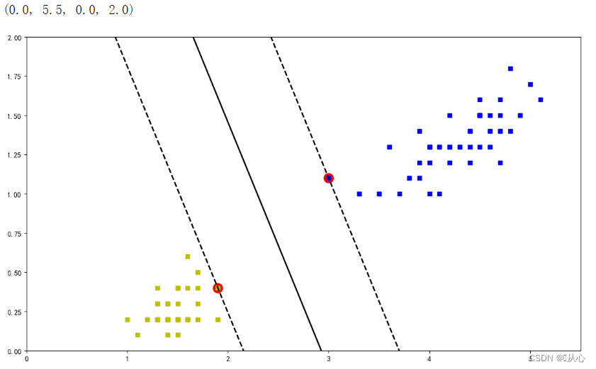

3、线性SVM（软间隔）流程

 3.1、获取数据

from sklearn.datasets import load_iris
from sklearn.model_selection import train_test_split

from sklearn.svm import SVC

# 获取数据
iris = load_iris()

3.2、数据预处理

x=iris.data[:,(2,3)]
y=(iris.target==2).astype(np.float64)

3.3、特征工程

3.4、模型训练

实现线性SVM用LinearSVC试试

from sklearn.pipeline import Pipeline
from sklearn.preprocessing import StandardScaler

svm_clf=Pipeline((
    ('std',StandardScaler()),
    ('linear_svc',LinearSVC(C = 1))
))

svm_clf.fit(x,y)

3.5、模型评估

3.6、结果预测

经过模型评估后通过的模型可以代入真实值进行预测。

svm_clf.predict([[5.5,1.7]])

3.7、可视化（不同C值带来的效果差异）

scaler = StandardScaler()

svm_clf1=SVC(kernel='linear',C=1,random_state=1473)
svm_clf2=SVC(kernel='linear',C=100,random_state=1473)

# scaled_svm_clf1=Pipeline((
#     ('std',StandardScaler()),
#     ('linear_svc',svm_clf1)
# ))

# scaled_svm_clf2=Pipeline((
#     ('std',StandardScaler()),
#     ('linear_svc',svm_clf2)
# ))
# scaled_svm_clf1.fit(x,y)

# scaled_svm_clf2.fit(x,y)

svm_clf1.fit(x,y)
svm_clf2.fit(x,y)

# 绘制决策边界
def plot_svc_decision_boundary(clf,sv=True):
    w=clf.coef_[0]
    b=clf.intercept_[0]

    x0=np.linspace(0,5.5,200)

    decision_boundary=-w[0]/w[1]*x0-b/w[1]
    margin=1/w[1]

    gutter_up=decision_boundary+margin
    gutter_down=decision_boundary-margin
    
    if sv:
        svs=clf.support_vectors_
        plt.scatter(svs[:,0],svs[:,1],s=180,facecolors='red')
    plt.plot(x0,decision_boundary,'k-',linewidth=2)
    plt.plot(x0,gutter_up,'k--',linewidth=2)
    plt.plot(x0,gutter_down,'k--',linewidth=2)

plt.figure(figsize=(14,4))

plt.subplot(121)
# 数据点
plt.plot(x[:,0][y==1],x[:,1][y==1],'bs',label="Iris-Virginica")
plt.plot(x[:,0][y==0],x[:,1][y==0],'ys',label="Iris-Versicolor")

# 决策边界和决策超平面
plot_svc_decision_boundary(svm_clf1,sv=True)
plt.xlabel("Petal length",fontsize=14)
plt.ylabel("Petal width",fontsize=14)
plt.legend(loc="upper left",fontsize=14)
plt.title("$C={}$".format(svm_clf1.C),fontsize=16)

plt.axis([4,6,0.5,3])


plt.subplot(122)
# 数据点
plt.plot(x[:,0][y==1],x[:,1][y==1],'bs',label="Iris-Virginica")
plt.plot(x[:,0][y==0],x[:,1][y==0],'ys',label="Iris-Versicolor")

# 决策边界和决策超平面
plot_svc_decision_boundary(svm_clf2,sv=True)
plt.xlabel("Petal length",fontsize=14)
plt.ylabel("Petal width",fontsize=14)
plt.legend(loc="upper left",fontsize=14)
plt.title("$C={}$".format(svm_clf2.C),fontsize=16)

plt.axis([4,6,0.5,3])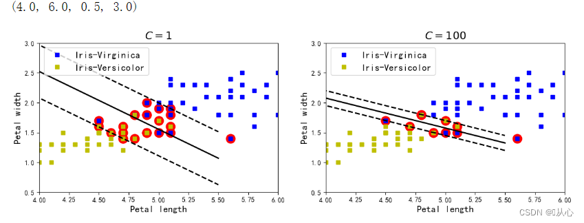

 4、非线性可分SVM（核技巧）

4.1、升维转换演示

x1D=np.linspace(-4,4,9).reshape(-1,1)
x2D=np.c_[x1D,x1D**2]
y=np.array([0,0,1,1,1,1,1,0,0])

plt.figure(figsize=(11,4))

plt.subplot(121)

plt.grid(True,which='both')
plt.axhline(y=0,color='k')
plt.plot(x1D[:,0][y==0],np.zeros(4),'bs')
plt.plot(x1D[:,0][y==1],np.zeros(5),'g^')
plt.gca().get_yaxis().set_ticks([])
plt.xlabel(r"$x_1$",fontsize=20)
plt.axis([-4.5,4.5,-0.2,0.2])
np.zeros(4)

x1D=np.linspace(-4,4,9).reshape(-1,1)
x2D=np.c_[x1D,x1D**2]
y=np.array([0,0,1,1,1,1,1,0,0])

plt.figure(figsize=(11,4))

plt.subplot(121)

plt.grid(True,which='both')
plt.axhline(y=0,color='k')
plt.plot(x1D[:,0][y==0],np.zeros(4),'bs')
plt.plot(x1D[:,0][y==1],np.zeros(5),'g^')
plt.gca().get_yaxis().set_ticks([])
plt.xlabel(r"$x_1$",fontsize=20)
plt.axis([-4.5,4.5,-0.2,0.2])
np.zeros(4)


plt.subplot(122)
plt.grid(True,which='both')
plt.axhline(y=0,color='k')
plt.axvline(x=0,color='k')
plt.plot(x2D[:,0][y==0],x2D[:,1][y==0],'bs')
plt.plot(x2D[:,0][y==1],x2D[:,1][y==1],'g^')
plt.xlabel(r"$x_1$",fontsize=20)
plt.xlabel(r"$x_2$",fontsize=20,rotation=0)
plt.gca().get_yaxis().set_ticks([0,4,8,12,16])
plt.plot([-4.5,4.5],[6.5,6.5],'r--',linewidth=3)
plt.axis([-4.5,4.5,-1,17])

plt.subplots_adjust(right=1)
plt.show()

4.2、线性核

4.2.1、创建非线性数据

from sklearn.datasets import make_moons
x,y=make_moons(n_samples=100,noise=0.15,random_state=1473)

# 创建非线性数据
def plot_dataset(x,y,axes):
    plt.plot(x[:,0][y==0],x[:,1][y==0],'bs')
    plt.plot(x[:,0][y==1],x[:,1][y==1],'g^')
    plt.axis(axes)
    plt.grid(True,which='both')
    plt.xlabel(r"$x_1$",fontsize=20)
    plt.xlabel(r"$x_2$",fontsize=20,rotation=0)
    
plot_dataset(x,y,[-1.5,2.5,-1,1.5])
plt.show()

4.2.2、分类预测

使用PolynomialFeatures模块进行预处理，使用这个可以增加数据维度
polynomial_svm_clf.fit(X,y)对当前进行训练传进去X和y数据

# 分类预测
from sklearn.datasets import make_moons
from sklearn.pipeline import Pipeline
from sklearn.preprocessing import PolynomialFeatures

polynomial_svm_clf=Pipeline((("poly_features",PolynomialFeatures(degree=3)),
                            ("scaler" ,StandardScaler()),
                            ("svm_clf",LinearSVC(C=10,loss="hinge"))))


polynomial_svm_clf.fit(x,y)

def plot_predictions(clf,axes):
    x0s=np.linspace(axes[0],axes[1],100)
    x1s=np.linspace(axes[2],axes[3],100)
    x0,x1=np.meshgrid(x0s,x1s)
    x=np.c_[x0.ravel(),x1.ravel()]
    y_pred=clf.predict(x).reshape(x0.shape)
    plt.contourf(x0,x1,y_pred,cmap=plt.cm.brg,alpha=0.2)
    
plot_predictions(polynomial_svm_clf,[-1.5,2.5,-1,1.5])
plot_dataset(x,y,[-1.5,2.5,-1,1.5])

4.3、多项式核函数

poly_kernel_svm_clf=Pipeline([
    ("scaler",StandardScaler()),
    ("svm_clf",SVC(kernel='poly',degree=3,coef0=1,C=5))
])

poly_kernel_svm_clf.fit(x,y)

poly100_kernel_svm_clf=Pipeline([
    ("scaler",StandardScaler()),
    ("svm_clf",SVC(kernel='poly',degree=10,coef0=100,C=5))
])

poly100_kernel_svm_clf.fit(x,y)

plt.figure(figsize=(11,4))

plt.subplot(121)
plot_predictions(poly_kernel_svm_clf,[-1.5,2.5,-1,1.5])
plot_dataset(x,y,[-1.5,2.5,-1,1.5])
plt.title(r"$d=3,r=1,C=5$")

plt.subplot(122)
plot_predictions(poly100_kernel_svm_clf,[-1.5,2.5,-1,1.5])
plot_dataset(x,y,[-1.5,2.5,-1,1.5])
plt.title(r"$d=10,r=100,C=5$")

plt.show()

 4.4、高斯(径向基)RBF核函数

import numpy as np
from matplotlib import pyplot as plt
 
## 构造数据
X1D = np.linspace(-4, 4, 9).reshape(-1, 1)
X2D = np.c_[X1D, X1D ** 2]
y = np.array([0, 0, 1, 1, 1, 1, 1, 0, 0])
from sklearn.datasets import make_moons
 
    
X, y = make_moons(n_samples=100, noise=0.15, random_state=42)  #指定两个环形测试数据
 
from sklearn.svm import SVC
from sklearn.pipeline import Pipeline  ##使用操作流水线
from sklearn.preprocessing import StandardScaler

## 通过设置degree值来进行对比实验
poly_kernel_svm_clf = Pipeline([
    ("scaler", StandardScaler()),
    ("svm_clf", SVC(kernel="poly", degree=3, coef0=1, C=5))  ##coef0表示偏置项
])
poly_kernel_svm_clf.fit(X, y)
 
poly100_kernel_svm_clf = Pipeline([
    ("scaler", StandardScaler()),
    ("svm_clf", SVC(kernel="poly", degree=100, coef0=1, C=5))
])
poly100_kernel_svm_clf.fit(X, y)
 
# 制图展示对比结果
def plot_predictions(clf, axes):
    xOs = np.linspace(axes[0], axes[1], 100)
    x1s = np.linspace(axes[2], axes[3], 100)
    x0, x1 = np.meshgrid(xOs, x1s)  ##构建坐标棋盘
    X = np.c_[x0.ravel(), x1.ravel()]
    y_pred = clf.predict(X).reshape(x0.shape)  #一定要对预测结果进行reshape操作
    plt.contourf(x0, x1, y_pred, cmap=plt.cm.brg, alpha=0.2)
 
 
def plot_dataset(X, y, axes):
    plt.plot(X[:, 0][y == 0], X[:, 1][y == 0], "bs")
    plt.plot(X[:, 0][y == 1], X[:, 1][y == 1], "g^")
    plt.axis(axes)
    plt.grid(True, which='both')
    plt.xlabel(r"$x_1$", fontsize=20)
    plt.ylabel(r"$x_2$", fontsize=20, rotation=0)
 
 
plt.figure(figsize=(11, 4))
plt.subplot(121)
plot_predictions(poly_kernel_svm_clf, [-1.5, 2.5, -1, 1.5])
plot_dataset(X, y, [-1.5, 2.5, -1, 1.5])
plt.title(r"$d=3,r=1,C=5$", fontsize=18)
plt.subplot(122)
plot_predictions(poly100_kernel_svm_clf, [-1.5, 2.5, -1, 1.5])
plot_dataset(X, y, [-1.5, 2.5, -1, 1.5])
plt.title(r"$d=10,r=100,C=5$", fontsize=18)
plt.show()

# 定义高斯核函数
def gaussian_rbf(x, landmark, gamma):
    '''
    :param x: 待变换数据
    :param landmark:当前选择位置
    :param gamma:（不同γ值对公式会产生不同的影响）
    :return:
    '''
    return np.exp(-gamma * np.linalg.norm(x - landmark, axis=1) ** 2)

gamma = 0.3

x1s = np.linspace(-4.5, 4.5, 200).reshape(-1, 1)
##分别选择不同的地标将数据进行映射
x2s = gaussian_rbf(x1s, -2, gamma)
x3s = gaussian_rbf(x1s, 1, gamma)
 
XK = np.c_[gaussian_rbf(X1D, -2, gamma), gaussian_rbf(X1D, 1, gamma)]
yk = np.array([0, 0, 1, 1, 1, 1, 1, 0, 0])
 
plt.figure(figsize=(11, 4))

###绘制变换前数据分布已经变换过程
plt.subplot(121)
plt.grid(True, which='both')
plt.axhline(y=0, color='k')
plt.scatter(x=[-2, 1], y=[0, 0], s=150, alpha=0.5, c="red")
plt.plot(X1D[:, 0][yk == 0], np.zeros(4), "bs")
plt.plot(X1D[:, 0][yk == 1],np.zeros(5), "g^")
plt.plot(x1s, x2s, "g-")
plt.plot(x1s, x3s, "b:")
plt.gca().get_yaxis().set_ticks([0, 0.25, 0.5, 0.75, 1])
plt.xlabel(r"$x_1$", fontsize=20)
plt.ylabel(r"Similarity", fontsize=14)
plt.annotate(r'$\mathbf{x}$',
             xy=(X1D[3, 0], 0),
             xytext=(-0.5, 0.20),
             ha="center",
             arrowprops=dict(facecolor='black', shrink=0.1),
             fontsize=18, )
plt.text(-2, 0.9, "Sx_2s", ha="center", fontsize=20)
plt.text(1, 0.9, "Sx_3S", ha="center", fontsize=20)
plt.axis([-4.5, 4.5, -0.1, 1.1])

###绘制最终结果与分界线
plt.subplot(122)
plt.grid(True, which='both')
plt.axhline(y=0, color='k')
plt.axvline(x=0, color='k')
plt.plot(XK[:, 0][yk == 0], XK[:, 1][yk == 0], "bs")
plt.plot(XK[:, 0][yk == 1], XK[:, 1][yk == 1], "g^")
plt.xlabel(r"$x_2$", fontsize=20)
plt.ylabel(r"$x_3$", fontsize=20, rotation=0)
plt.annotate(r'$\phi\left (\mathbf{x}\right)$',
             xy=(XK[3, 0], XK[3, 1]),
             xytext=(0.65, 0.50),
             ha="center",
             arrowprops=dict(facecolor='black', shrink=0.1),
             fontsize=18, )
plt.plot([-0.1, 1.1], [0.57, -0.1], "r--", linewidth=3)
plt.axis([-0.1, 1.1, -0.1, 1.1])
 
plt.subplots_adjust(right=1)
 
plt.show()

### 探讨γ值与C值对模型结果的影响'''
from sklearn.svm import SVC
 
gamma1, gamma2 = 0.1, 5
C1, C2 = 0.001, 1000
hyperparams = (gamma1, C1), (gamma1, C2), (gamma2, C1), (gamma2, C2)
 
svm_clfs = []
for gamma, C in hyperparams:
    rbf_kernel_svm_clf = Pipeline([
        ("scaler", StandardScaler()),
        ("svm_clf", SVC(kernel="rbf", gamma=gamma, C=C))
    ])
    rbf_kernel_svm_clf.fit(X, y)
    svm_clfs.append(rbf_kernel_svm_clf)
plt.figure(figsize=(11, 7))
 
for i, svm_clf in enumerate(svm_clfs):
    plt.subplot(221 + i)
    plot_predictions(svm_clf, [-1.5, 2.5, -1, 1.5])
    plot_dataset(X, y, [-1.5, 2.5, -1, 1.5])
    gamma, C = hyperparams[i]
    plt.title(r'$\gamma={},C={}$'.format(gamma, C), fontsize=16)
plt.show()

旧梦可以重温，且看：机器学习（五） -- 监督学习（7） --SVM1
欲知后事如何，且看：