在深度学习的优化过程中,梯度下降法及其变体是必不可少的工具。通过对梯度下降法的理论学习,我们能够更好地理解深度学习模型的训练过程。本篇文章将介绍梯度下降的基本原理,并通过代码实现展示其具体应用。我们会从二维平面的简单梯度下降开始,逐步过渡到三维,再对比多种优化器的效果。
一、梯度下降法简介
梯度下降法(Gradient Descent)是一种常用的优化算法,广泛应用于机器学习和深度学习中。其基本思想是通过迭代更新参数,使得损失函数逐步减小,最终找到最优解。常见的梯度下降法包括随机梯度下降(SGD)、动量法(Momentum)、自适应学习率方法(Adagrad、RMSprop、Adadelta)和Adam等。
二、梯度下降的二维实现
首先,我们来实现一个简单的二维平面内的梯度下降法。目标是找到函数 \(f(x) = x^2 + 4x + 1\) 的最小值。
import torch
import matplotlib.pyplot as plt
# 定义目标函数
def f(x):
return x**2 + 4*x + 1
# 初始化参数
x = torch.tensor([2.0], requires_grad=True)
learning_rate = 0.7
# 记录每次梯度下降的值
xs, ys = [], []
# 梯度下降迭代
for i in range(100):
y = f(x)
y.backward()
with torch.no_grad():
x -= learning_rate * x.grad
x.grad.zero_()
xs.append(x.item())
ys.append(y.item())
# 打印最终结果
print(f"最终x值: {x.item()}")
# 可视化
x_vals = torch.linspace(-4, 2, 100)
y_vals = f(x_vals)
plt.plot(x_vals.numpy(), y_vals.numpy(), label='f(x)=x^2 + 4x + 1')
plt.scatter(xs, ys, color='red', label='Gradient Descent')
plt.xlabel('x')
plt.ylabel('f(x)')
plt.legend()
plt.show()通过以上代码,我们能够看到从初始点出发,梯度下降法逐步逼近最小值。
三、梯度下降的三维实现
增加一个维度,函数变为 \(f(x, y) = x^2 + y^2\),我们希望通过梯度下降法找到该函数的最小值。
from mpl_toolkits.mplot3d import Axes3D

# 定义目标函数
def f(x, y):
    return x**2 + y**2

# 初始化参数
x = torch.tensor([2.0], requires_grad=True)
y = torch.tensor([2.0], requires_grad=True)
learning_rate = 0.1

# 记录每次梯度下降的值
xs, ys, zs = [], [], []

# 梯度下降迭代
for i in range(100):
    z = f(x, y)
    z.backward()

    with torch.no_grad():
        x -= learning_rate * x.grad
        y -= learning_rate * y.grad
        x.grad.zero_()
        y.grad.zero_()

    xs.append(x.item())
    ys.append(y.item())
    zs.append(z.item())

# 打印最终结果
print(f"最终x, y值: {x.item()}, {y.item()}")

# 可视化
fig = plt.figure()
ax = fig.add_subplot(111, projection='3d')
ax.plot(xs, ys, zs, label='Gradient Descent Path', marker='o')
ax.set_xlabel('X')
ax.set_ylabel('Y')
ax.set_zlabel('Z')
plt.legend()
plt.show()

# 等高线图
plt.figure()
X, Y = torch.meshgrid(torch.linspace(-3, 3, 100), torch.linspace(-3, 3, 100))
Z = f(X, Y)
plt.contourf(X.numpy(), Y.numpy(), Z.numpy(), 50)
plt.plot(xs, ys, 'r-o', label='Gradient Descent Path')
plt.xlabel('x')
plt.ylabel('y')
plt.legend()
plt.show()
通过以上代码,我们能够在三维空间中看到梯度下降的路径。
四、不同优化器的对比
接下来,我们生成一个数据集,使用不同的优化器进行对比,观察它们的收敛效果。
import torch.utils.data as data

# 生成数据集
def generate_data(num_samples=1000):
    x = torch.rand(num_samples, 1)
    y = torch.rand(num_samples, 1)
    z = f(x, y) + torch.randn(num_samples, 1)
    return x, y, z

x, y, z = generate_data()
dataset = data.TensorDataset(torch.cat([x, y], dim=1), z)
train_size = int(0.8 * len(dataset))
test_size = len(dataset) - train_size
train_dataset, test_dataset = data.random_split(dataset, [train_size, test_size])
train_loader = data.DataLoader(train_dataset, batch_size=32)
test_loader = data.DataLoader(test_dataset, batch_size=32)

# 定义模型
class SimpleNN(torch.nn.Module):
    def __init__(self):
        super(SimpleNN, self).__init__()
        self.fc = torch.nn.Linear(2, 1)

    def forward(self, x):
        return self.fc(x)

# 初始化模型和优化器
models = [SimpleNN() for _ in range(6)]
optimizers = [
    torch.optim.SGD(models[0].parameters(), lr=0.01),
    torch.optim.SGD(models[1].parameters(), lr=0.01, momentum=0.9),
    torch.optim.Adagrad(models[2].parameters(), lr=0.01),
    torch.optim.RMSprop(models[3].parameters(), lr=0.01),
    torch.optim.Adadelta(models[4].parameters()),
    torch.optim.Adam(models[5].parameters(), lr=0.01)
]
loss_fn = torch.nn.MSELoss()

# 训练和测试函数
def train_epoch(model, optimizer, loader):
    model.train()
    total_loss = 0
    for x_batch, y_batch in loader:
        optimizer.zero_grad()
        y_pred = model(x_batch)
        loss = loss_fn(y_pred, y_batch)
        loss.backward()
        optimizer.step()
        total_loss += loss.item()
    return total_loss / len(loader)

def test_epoch(model, loader):
    model.eval()
    total_loss = 0
    with torch.no_grad():
        for x_batch, y_batch in loader:
            y_pred = model(x_batch)
            loss = loss_fn(y_pred, y_batch)
            total_loss += loss.item()
    return total_loss / len(loader)

# 记录误差
train_losses = [[] for _ in range(6)]
test_losses = [[] for _ in range(6)]

# 训练和测试过程
num_epochs = 50
for epoch in range(num_epochs):
    for i in range(6):
        train_loss = train_epoch(models[i], optimizers[i], train_loader)
        test_loss = test_epoch(models[i], test_loader)
        train_losses[i].append(train_loss)
        test_losses[i].append(test_loss)

# 可视化收敛曲线
plt.figure(figsize=(12, 6))
for i, name in enumerate(['SGD', 'Momentum', 'Adagrad', 'RMSprop', 'Adadelta', 'Adam']):
    plt.plot(train_losses[i], label=f'Train {name}')
    plt.plot(test_losses[i], '--', label=f'Test {name}')
plt.xlabel('Epoch')
plt.ylabel('Loss')
plt.legend()
plt.show()
通过上述代码,我们能够对比不同优化器的收敛效果,从图中可以看到各个优化器的表现差异。
五、总结
本文通过代码实现详细展示了梯度下降法在二维和三维空间中的应用,并对比了多种优化器的效果。通过这些实践,我们能够更直观地理解梯度下降法的工作原理及其在深度学习中的应用。希望大家通过本篇文章,能够更加熟练地应用梯度下降及其变体进行模型训练。加油!