神经网络-万能近似定理的探索

神经网络-万能近似定理的探索

对于这个实验博主想说，其实真的很有必要去好好做一下，很重要的一个实验。

1.理论介绍

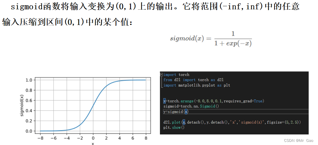
万能近似定理: ⼀个前馈神经⽹络如果具有线性层和⾄少⼀层具有 “挤压” 性质的激活函数（如 sigmoid 等），给定⽹络⾜够数量的隐藏单元，它可以以任意精度来近似任何从⼀个有限维空间到另⼀个有限维空间的 borel 可测函数。

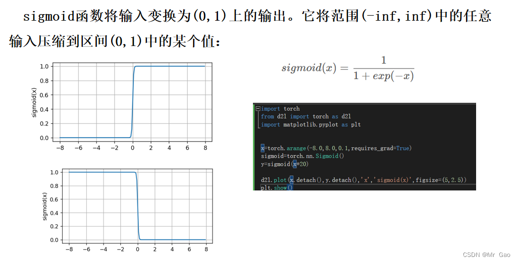
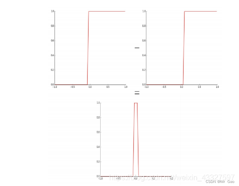
我们可以通过两个 sigmoid 函数 (y = sigmoid(w⊤x + b)) ⽣成⼀个 tower，如图：

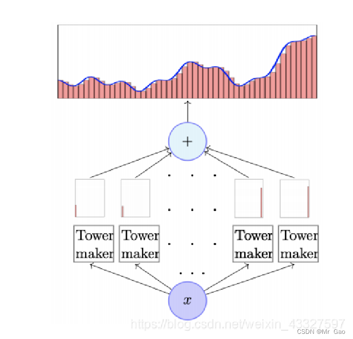
我们构造多个这样的 tower 近似任意函数：

2.数据集介绍

使用PyTorch库来执行数值计算，首先通过 torch.linspace 函数创建了一个从0到3的等差数列，其元素数量由变量 sample_num 决定。接着定义了一个多项式函数 function，它接受一个参数 x 并返回 x + x**3 + 3 的值。最后，代码通过将 x_data 作为输入应用 function 函数，计算并存储了每个数据点对应的函数值到 y_real 变量中，从而实现了对一系列数据点的生成。

sample_num=300
torch.manual_seed(10)

x_data=torch.linspace(0,3,sample_num)


def function(x):
  return x+x**3+3



y_real=function(x_data)

3.实验过程

所有代码如下：

#coding=gbk

import torch
from torch.autograd import Variable
from torch.utils import data
import matplotlib.pyplot as plt

neuron_num=200
batch=50
learn_rating=0.005
epoch=1000


#print(x_data)

sample_num=50
torch.manual_seed(10)

x_data=torch.linspace(0,3,sample_num)


def function(x):
  return x+x**3+3



y_real=function(x_data)
#print(y_real)

wz=torch.rand(neuron_num)
#print(wz)
w=torch.normal(0,1,size=(neuron_num,))
b=torch.normal(0,1,size=(neuron_num,))
w2=torch.normal(0,1,size=(neuron_num,))
b2=torch.normal(0,1,size=(1,))
#print(w,b)


def sampling(sample_num):
   
    #print(data_size)
    index_sequense=torch.randperm(sample_num)
    return index_sequense
def activation_function(x):
    return 1/(1+torch.sigmoid(-x))


def activation_function2(x):
   
   # print(x.size())
    a=torch.rand(x.size())
    for i in range(x.size(0)):
        if x[i]<=0:
            a[i]=0.0
        else:
            a[i]=x[i]
    return a
def hidden_layer(w,b,x):
   # print("x:",x)
    return activation_function2(w*x+b)

def  fully_connected_layer(w2,b2,x):
    return torch.dot(w2,x)+b2

def net(w,b,w2,b2,x):
    #print("w",w)
    #print("b",b)
    o1=hidden_layer(w,b,x)
    #print("o1",o1)
    #print("w2",w2)
    #print("b2",b2)
    o2=fully_connected_layer(w2,b2,o1)
 #   print("o2",o2)

    return o2

def get_grad(w,b,w2,b2,x,y_predict,y_real):
  

    o2=hidden_layer(w,b,x)

    l_of_w2=-(y_real-y_predict)*o2
    l_of_b2=-(y_real-y_predict)

    a=torch.rand(o2.size())
    for i in range(o2.size(0)):
        if o2[i]<=0:
            a[i]=0.0
        else:
            a[i]=1
    l_of_w=-(y_real-y_predict)*torch.dot(w2,a)*x
    l_of_b=-(y_real-y_predict)*torch.dot(w2,a)

    return l_of_w2,l_of_b2,l_of_w,l_of_b

def loss_function(y_predict,y_real):
    #print(y_predict,y_real)
    return torch.pow(y_predict-y_real,2)
loss_list=[]

torch.device("cuda:0" if torch.cuda.is_available() else "cpu")

device = torch.device("cuda" if torch.cuda.is_available() else "cpu")

def train():
    global w,w2,b,b2
    index=0
    index_sequense=sampling(sample_num)
    for i in range(epoch):
        
        
   
        W_g=torch.zeros(neuron_num)
        b_g=torch.zeros(neuron_num)
        W2_g=torch.zeros(neuron_num)
        b2_g=torch.zeros(1)
        loss=torch.tensor([0.0])
           
        for k in range(batch):
              try:
                   # print("x",x_data[index],index)
                   # print("w",w)
                        y_predict=net(w,b,w2,b2,x_data[index_sequense[index]])

                        get_grad(w,b,w2,b2,x_data[index_sequense[index]],y_predict,y_real[index_sequense[index]])
                      
                        l_of_w2,l_of_b2,l_of_w,l_of_b= get_grad(w,b,w2,b2,x_data[index_sequense[index]],y_predict,y_real[index_sequense[index]])
                        W_g=W_g+l_of_w
                        b_g=b_g+l_of_b
                        b2_g=b2_g+l_of_b2
                        W2_g=W2_g+l_of_w2
                        loss=loss+loss_function(y_predict,y_real[index_sequense[index]])
                        index=index+1
              except:
                        index=0
                      #  index_sequense=sampling(sample_num)
        print("****************************loss is :",loss/batch)
        loss_list.append(loss/batch)
     
        W_g=W_g/batch
        b_g=b_g/batch
        b2_g=b2_g/batch
        W2_g=W2_g/batch
        w=w-learn_rating*W_g
        b=b-learn_rating*b_g
        w2=w2-learn_rating*W2_g
        b2=b2-learn_rating*b2_g
y_predict=net(w,b,w2,b2,x_data[0])
train()
y_predict=[]
for i in range(sample_num):
  y_predict.append(net(w,b,w2,b2,x_data[i]))

epoch_list=list(range(epoch))
plt.plot(epoch_list,loss_list,label='SGD')
plt.title("loss")
plt.legend()

plt.show()

plt.plot(x_data,y_real,label='real')
plt.plot(x_data,y_predict,label='predict')
plt.title(" Universal Theorem of Neural Networks")
plt.legend()
plt.show()
print(w,b,w2,b2)

4.总结

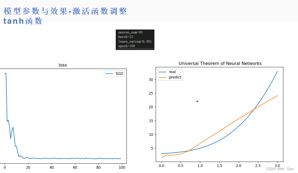
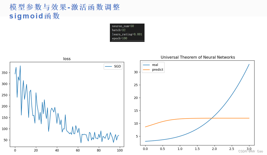
（1）相比较之下，tanh函数比sigmoid函数效果要好很多，但是如果，神经元数量足够，训练足够充分，两者效果会差不多。在训练不够充分，神经元不够多，学习率等条件限制下，tanh函数表现更好。
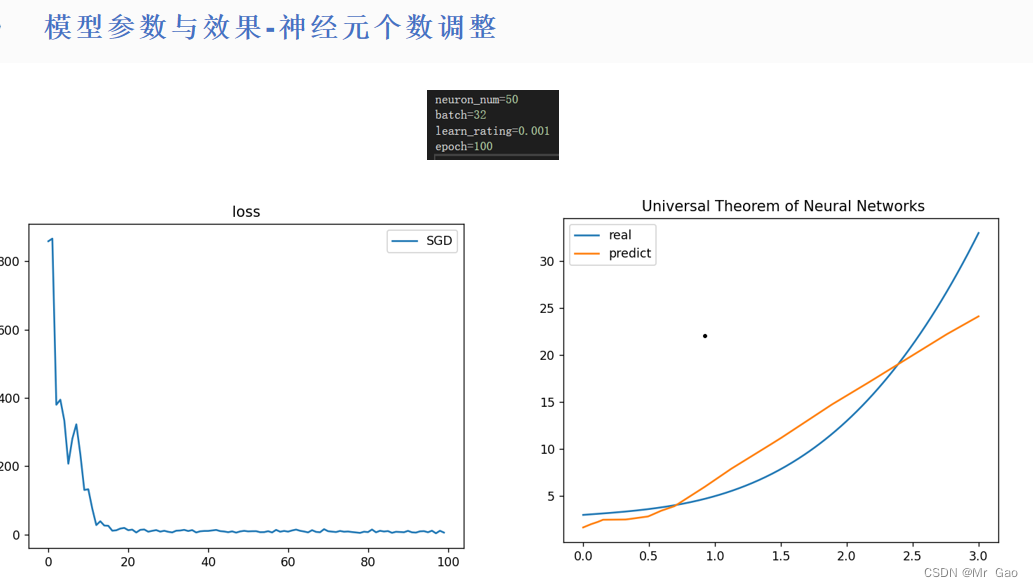
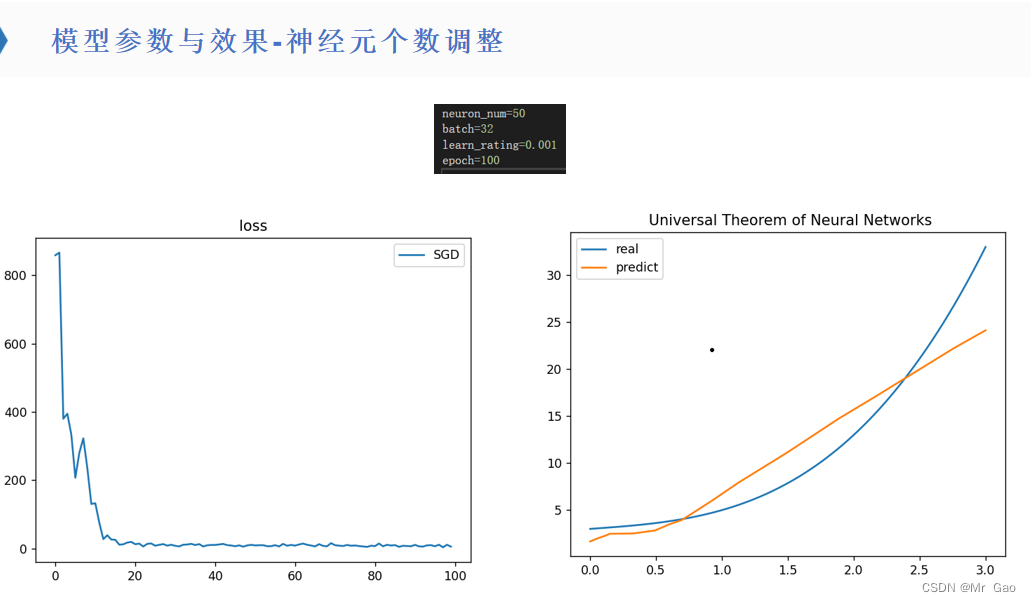
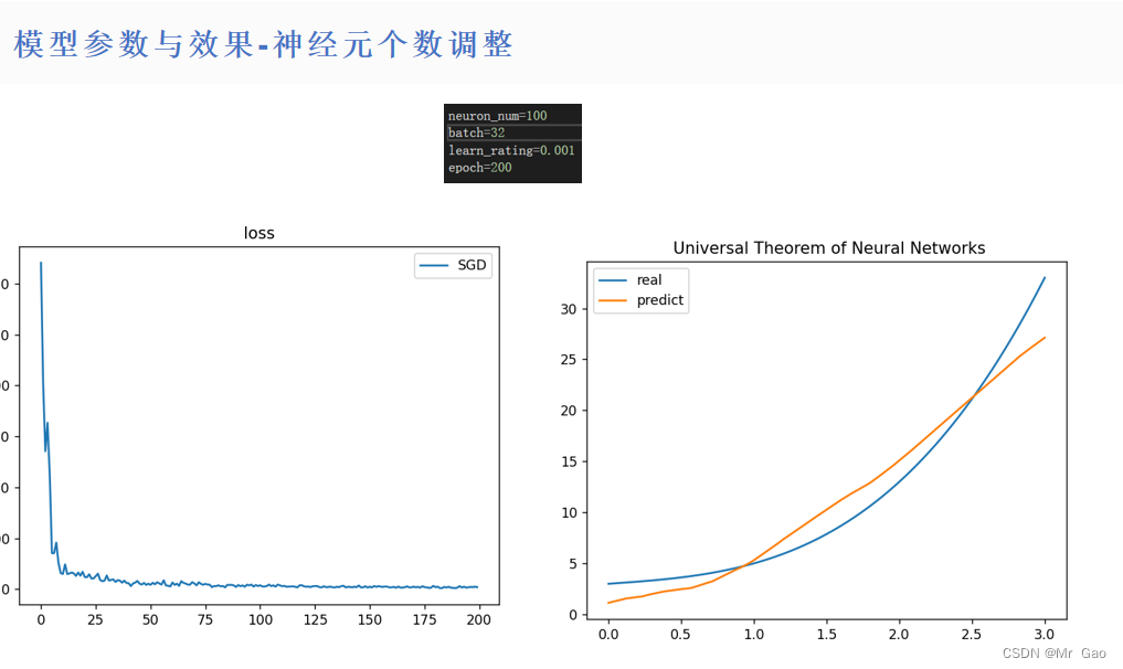
（2）神经元数量越多的情况下，模型性能在不断提升，但是学习越来越慢，如果采用随机梯度下降或者小批量梯度下降，最好增加神经元，否则，学习最终性能会受到很大限制。
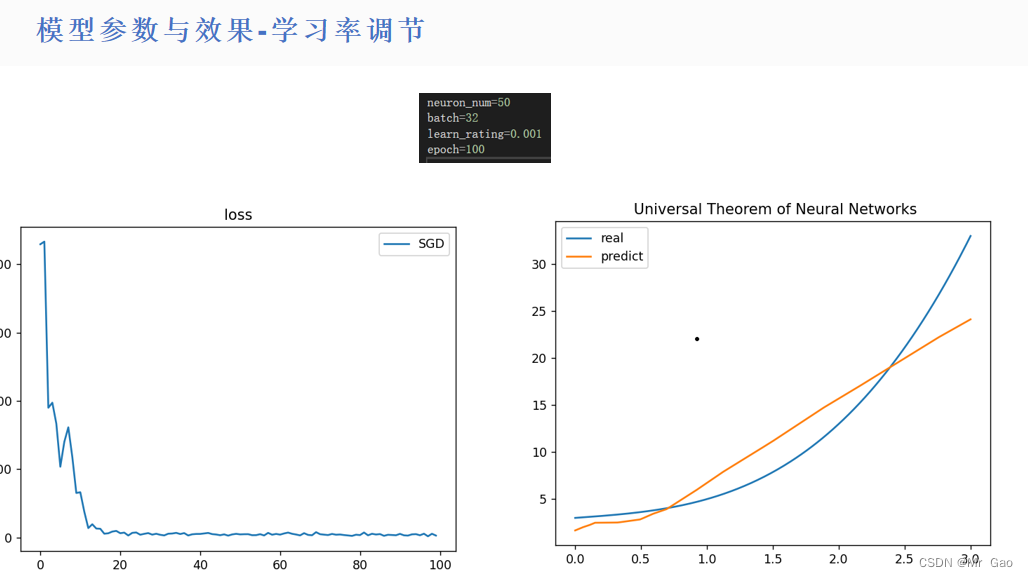
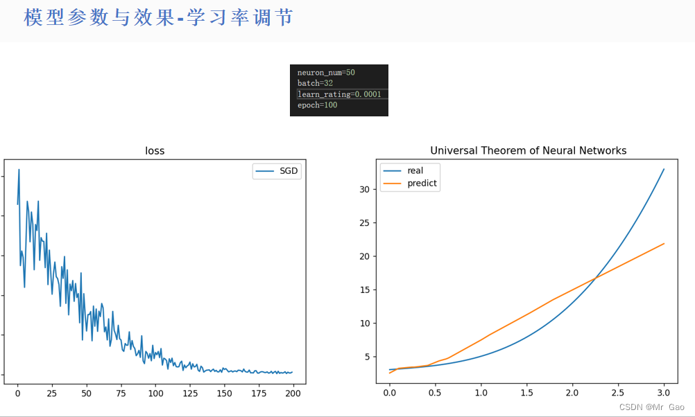
（3）对于不同数量的神经元，最优学习率是在变化的。
（4）如果采用随机梯度下降或者小批量梯度下降，样本不能反应总体规律，那么网络要足够大，才能进行规律的总结，否则，最好采用批量梯度下降去处理问题。
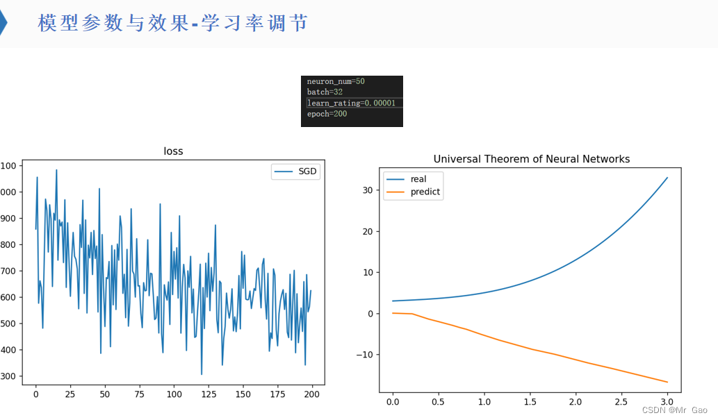
（5）不同的超参数设置，最终学习的性能会有瓶颈，需要进行学习策略，超参数的调节，才能不断提高模型效果。