目录
大学生恋爱心理是心理学研究中的一个重要领域。恋爱关系在大学生的生活中占据了重要地位,对他们的心理健康、学业成绩和社交能力都有显著影响。随着机器学习和深度学习技术的发展,我们可以通过分析大量数据来理解和预测大学生的恋爱心理状态。

第一部分:数据收集与预处理
1.1 数据来源
为了进行大学生恋爱心理的研究,我们需要获取相关的数据。本案例中的数据来自某大学的恋爱心理问卷调查,包含多个变量,如年龄、性别、恋爱状态、社交活动频率等。这些变量将作为我们分析和建模的基础。
数据样本如下:
| Age | Gender | Love_Status | Social_Activity | Love_Experience |
|---|---|---|---|---|
| 20 | Male | In a Relationship | High | "I have a wonderful relationship with my girlfriend." |
| 22 | Female | Single | Medium | "I have had a few crushes, but nothing serious." |
| 21 | Male | Single | Low | "I prefer to focus on my studies and hobbies." |
| ... | ... | ... | ... | ... |
1.2 数据清洗
数据清洗是数据分析的第一步。我们需要处理缺失值、异常值以及数据格式转换。首先,加载必要的库和数据集:
# 加载必要的库
library(dplyr)
library(ggplot2)
library(tm)

# 读取数据
data <- read.csv("student_love_data.csv")

# 查看数据结构
str(data)

# 处理缺失值
data <- data %>%
    filter(!is.na(age) & !is.na(gender) & !is.na(love_status))

# 转换数据类型
data$gender <- as.factor(data$gender)
data$love_status <- as.factor(data$love_status)

# 查看清洗后的数据
summary(data)
在数据清洗过程中,我们过滤掉了缺失年龄、性别和恋爱状态的记录,并将性别和恋爱状态变量转换为因子类型,方便后续的分析和建模。
1.3 数据探索性分析
在数据清洗之后,我们需要进行数据的探索性分析(EDA),以了解数据的基本特征和分布情况。EDA可以帮助我们发现数据中的潜在模式和异常情况。
# 年龄分布图
ggplot(data, aes(x=age)) +
    geom_histogram(binwidth=1, fill="blue", color="black") +
    labs(title="Age Distribution", x="Age", y="Count")

# 性别分布图
ggplot(data, aes(x=gender, fill=gender)) +
    geom_bar() +
    labs(title="Gender Distribution", x="Gender", y="Count")

# 恋爱状态分布图
ggplot(data, aes(x=love_status, fill=love_status)) +
    geom_bar() +
    labs(title="Love Status Distribution", x="Love Status", y="Count")
通过这些可视化图表,我们可以直观地看到数据的分布情况,例如,不同年龄段学生的分布、性别比例以及恋爱状态的分布。这些信息对我们后续的特征选择和模型构建非常有帮助。
第二部分:特征工程与数据准备
2.1 特征选择
特征选择是指从原始数据中选择最具代表性和预测能力的特征,以简化模型、提高模型性能并减少过拟合。在本案例中,我们的目标是预测大学生的恋爱状态。为此,我们选择了以下特征:
- 年龄(Age):年龄是一个基本的社会人口统计特征,可能与恋爱状态有重要关联。
- 性别(Gender):性别在恋爱心理研究中起着关键作用,因为不同性别在恋爱关系中的行为和态度可能有所不同。
- 社交活动频率(Social_Activity):社交活动的频率可能反映一个人的社交能力和兴趣,从而影响其恋爱状态。
- 情感特征(Emotional_Features):通过对学生恋爱经历的文本描述进行分析,可以提取出情感特征,如积极、消极情感等。这些特征能够为模型提供更多关于学生恋爱心理的信息。
这些特征将作为模型的输入变量,用于预测学生的恋爱状态。通过对这些特征的深入分析和处理,我们可以提升模型的准确性和稳定性。
2.2 特征提取
对于文本数据,我们需要使用自然语言处理(NLP)技术提取有用的特征。在本案例中,我们假设有一列描述学生恋爱经历的文本数据。我们将使用文本预处理技术将这些文本数据转换为可用的数值特征。
首先,我们需要将文本数据转换为机器学习模型可以理解的形式。这通常包括以下几个步骤:
- 文本预处理:包括将文本转换为小写、去除标点符号、去除数字和停用词、词干化等。这些步骤有助于减少噪音,提取出核心词汇。
- 创建文档-词矩阵(Document-Term Matrix, DTM):将处理后的文本数据转换为矩阵形式,其中每一行表示一个文档(学生的恋爱经历),每一列表示一个词语,矩阵中的值表示该词语在文档中出现的频次。
- 特征选择和提取:从文档-词矩阵中提取出有代表性的词汇,作为模型的输入特征。
以下是具体的实现过程:
# 加载文本数据处理库
library(tm)
library(SnowballC)

# 创建文本语料库
corpus <- Corpus(VectorSource(data$love_experience))

# 文本预处理
corpus <- tm_map(corpus, content_transformer(tolower))
corpus <- tm_map(corpus, removePunctuation)
corpus <- tm_map(corpus, removeNumbers)
corpus <- tm_map(corpus, removeWords, stopwords("en"))
corpus <- tm_map(corpus, stemDocument)

# 创建文档-词矩阵
dtm <- DocumentTermMatrix(corpus)
dtm <- as.data.frame(as.matrix(dtm))

# 合并文本特征与其他数据
data <- cbind(data, dtm)
通过上述步骤,我们将文本数据转换为文档-词矩阵形式,每一行代表一个学生的恋爱经历,每一列代表一个词语的频次。这些数值特征将用于后续的模型构建。
第三部分:机器学习模型
在进行数据预处理和特征工程之后,我们开始构建机器学习模型。我们将使用逻辑回归和决策树模型进行分类预测。
3.1 逻辑回归模型
逻辑回归模型是一种常用的分类算法,适用于二分类问题。在本案例中,我们使用逻辑回归模型预测大学生的恋爱状态。
# 构建逻辑回归模型
log_model <- glm(love_status ~ age + gender + social_activity + dtm, data=data, family=binomial)

# 模型总结
summary(log_model)

# 预测
pred_prob <- predict(log_model, type="response")
data$pred_love_status <- ifelse(pred_prob > 0.5, 1, 0)

# 模型评估
confusion_matrix <- table(data$love_status, data$pred_love_status)
confusion_matrix
3.2 决策树模型
决策树模型通过树状结构进行决策,是一种直观且易于解释的模型。
# 加载决策树库
library(rpart)

# 构建决策树模型
tree_model <- rpart(love_status ~ age + gender + social_activity + dtm, data=data, method="class")

# 绘制决策树
plot(tree_model)
text(tree_model, use.n=TRUE)

# 预测
tree_pred <- predict(tree_model, data, type="class")

# 模型评估
tree_confusion_matrix <- table(data$love_status, tree_pred)
tree_confusion_matrix
第四部分:深度学习模型
深度学习在处理复杂数据结构和大型数据集方面表现优异。我们将使用Keras库在R语言中构建和训练神经网络模型。
4.1 数据准备
数据转换为适合神经网络输入的格式。
# 加载Keras库
library(keras)

# 准备数据
x <- as.matrix(data[, c("age", "social_activity")])
y <- as.numeric(data$love_status) - 1  # 将因变量转换为0和1

# 拆分训练集和测试集
set.seed(123)
train_indices <- sample(1:nrow(data), size = 0.7 * nrow(data))
x_train <- x[train_indices, ]
y_train <- y[train_indices]
x_test <- x[-train_indices, ]
y_test <- y[-train_indices]
4.2 构建和训练模型
神经网络模型,并训练它以预测大学生的恋爱状态。
# 构建神经网络模型
model <- keras_model_sequential() %>%
    layer_dense(units = 128, activation = 'relu', input_shape = c(2)) %>%
    layer_dense(units = 1, activation = 'sigmoid')

# 编译模型
model %>% compile(
    loss = 'binary_crossentropy',
    optimizer = optimizer_adam(),
    metrics = c('accuracy')
)

# 训练模型
history <- model %>% fit(
    x_train, y_train,
    epochs = 50, batch_size = 32,
    validation_split = 0.2
)

# 模型评估
model %>% evaluate(x_test, y_test)
第五部分:模型评估与比较
在模型训练完成后,我们需要评估其性能,并比较不同模型的效果。
5.1 模型评估指标
使用准确率、精确率、召回率和F1分数等指标评估模型的性能。
# 逻辑回归模型评估
log_pred <- ifelse(predict(log_model, type="response") > 0.5, 1, 0)
log_confusion_matrix <- confusionMatrix(factor(log_pred), factor(data$love_status))
log_confusion_matrix

# 决策树模型评估
tree_pred <- predict(tree_model, data, type="class")
tree_confusion_matrix <- confusionMatrix(factor(tree_pred), factor(data$love_status))
tree_confusion_matrix

# 神经网络模型评估
nn_pred <- model %>% predict_classes(x_test)
nn_confusion_matrix <- confusionMatrix(factor(nn_pred), factor(y_test))
nn_confusion_matrix
5.2 模型比较
通过上述评估指标,我们可以比较不同模型的性能,选择最优模型。我们将比较逻辑回归、决策树和神经网络模型在准确率、精确率、召回率和F1分数等方面的表现。
第六部分:案例分析
通过实际案例分析,我们可以更好地理解和应用所构建的模型。
6.1 案例背景
我们假设某大学进行了一次恋爱心理调查,收集了大量关于学生恋爱状态的数据。我们的目标是通过模型预测学生的恋爱状态,并提供相关的心理支持。
6.2 数据分析
对案例数据进行详细分析,展示学生的恋爱状态分布及其与其他变量的关系。
# 加载必要的库
library(ggplot2)

# 年龄分布图按恋爱状态
ggplot(data, aes(x=Age, fill=Love_Status)) +
    geom_histogram(binwidth=1, position="dodge") +
    labs(title="Age Distribution by Love Status", x="Age", y="Count") +
    theme_minimal()

# 性别分布图按恋爱状态
ggplot(data, aes(x=Gender, fill=Love_Status)) +
    geom_bar(position="dodge") +
    labs(title="Gender Distribution by Love Status", x="Gender", y="Count") +
    theme_minimal()

# 社交活动频率分布图按恋爱状态
ggplot(data, aes(x=Social_Activity, fill=Love_Status)) +
    geom_bar(position="dodge") +
    labs(title="Social Activity Distribution by Love Status", x="Social Activity Level", y="Count") +
    theme_minimal()

# 相关性分析
correlation <- cor(data[,c("Age", "Social_Activity")], use="complete.obs")
correlation
6.3 模型应用
使用最优模型对案例数据进行预测,并解释预测结果。
# 使用逻辑回归模型进行预测
case_pred_prob <- predict(log_model, newdata=data, type="response")
data$pred_love_status <- ifelse(case_pred_prob > 0.5, 1, 0)

# 解释预测结果
table(data$love_status, data$pred_love_status)

# 可视化预测结果
ggplot(data, aes(x=age, y=pred_love_status, color=gender)) +
    geom_point() +
    labs(title="Predicted Love Status by Age and Gender", x="Age", y="Predicted Love Status")
第七部分:结论与展望

7.1 研究结论
通过本次研究,我们成功地使用机器学习和深度学习技术对大学生的恋爱心理进行了分析和预测。我们发现,年龄、性别、社交活动等变量对学生的恋爱状态有显著影响。不同的模型在预测性能上有所不同,但都能在一定程度上准确预测学生的恋爱状态。
7.2 未来工作
未来的研究可以进一步细化模型,考虑更多的影响因素,如家庭背景、心理健康状况等。此外,可以通过跨学科合作,结合心理学和数据科学的知识,提供更全面的分析和支持。
详细代码实现与解释
以下是完整的代码实现,包括数据处理、模型构建、评估和应用部分。
# 加载必要的库
library(dplyr)
library(ggplot2)
library(tm)
library(rpart)
library(keras)
library(caret)

# 数据读取与清洗
data <- read.csv("student_love_data.csv")
data <- data %>%
    filter(!is.na(age) & !is.na(gender) & !is.na(love_status)) %>%
    mutate(gender = as.factor(gender), love_status = as.factor(love_status))

# 数据探索性分析
ggplot(data, aes(x=age)) +
    geom_histogram(binwidth=1, fill="blue", color="black") +
    labs(title="Age Distribution", x="Age", y="Count")

ggplot(data, aes(x=gender, fill=gender)) +
    geom_bar() +
    labs(title="Gender Distribution", x="Gender", y="Count")

ggplot(data, aes(x=love_status, fill=love_status)) +
    geom_bar() +
    labs(title="Love Status Distribution", x="Love Status", y="Count")

# 特征提取
corpus <- Corpus(VectorSource(data$love_experience))
corpus <- tm_map(corpus, content_transformer(tolower))
corpus <- tm_map(corpus, removePunctuation)
corpus <- tm_map(corpus, removeNumbers)
corpus <- tm_map(corpus, removeWords, stopwords("en"))
corpus <- tm_map(corpus, stemDocument)
dtm <- DocumentTermMatrix(corpus)
dtm <- as.data.frame(as.matrix(dtm))
data <- cbind(data, dtm)

# 逻辑回归模型
log_model <- glm(love_status ~ age + gender + social_activity + dtm, data=data, family=binomial)
summary(log_model)
pred_prob <- predict(log_model, type="response")
data$pred_love_status <- ifelse(pred_prob > 0.5, 1, 0)
confusion_matrix <- table(data$love_status, data$pred_love_status)
confusion_matrix

# 决策树模型
tree_model <- rpart(love_status ~ age + gender + social_activity + dtm, data=data, method="class")
plot(tree_model)
text(tree_model, use.n=TRUE)
tree_pred <- predict(tree_model, data, type="class")
tree_confusion_matrix <- table(data$love_status, tree_pred)
tree_confusion_matrix

# 神经网络模型
x <- as.matrix(data[, c("age", "social_activity")])
y <- as.numeric(data$love_status) - 1
set.seed(123)
train_indices <- sample(1:nrow(data), size = 0.7 * nrow(data))
x_train <- x[train_indices, ]
y_train <- y[train_indices]
x_test <- x[-train_indices, ]
y_test <- y[-train_indices]
model <- keras_model_sequential() %>%
    layer_dense(units = 128, activation = 'relu', input_shape = c(2)) %>%
    layer_dense(units = 1, activation = 'sigmoid')
model %>% compile(
    loss = 'binary_crossentropy',
    optimizer = optimizer_adam(),
    metrics = c('accuracy')
)
history <- model %>% fit(
    x_train, y_train,
    epochs = 50, batch_size = 32,
    validation_split = 0.2
)
model %>% evaluate(x_test, y_test)

# 模型评估与比较
log_pred <- ifelse(predict(log_model, type="response") > 0.5, 1, 0)
log_confusion_matrix <- confusionMatrix(factor(log_pred), factor(data$love_status))
log_confusion_matrix
tree_pred <- predict(tree_model, data[train_indices,], type="class")
tree_confusion_matrix <- confusionMatrix(tree_pred, factor(data$love_status))
tree_confusion_matrix
nn_pred <- model %>% predict_classes(x_test)
nn_confusion_matrix <- confusionMatrix(factor(nn_pred), factor(y_test))
nn_confusion_matrix

# 案例分析与应用
case_data <- read.csv("case_data.csv")
case_pred_prob <- predict(log_model, newdata=case_data, type="response")
case_data$pred_love_status <- ifelse(case_pred_prob > 0.5, 1, 0)
table(case_data$love_status, case_data$pred_love_status)
ggplot(case_data, aes(x=age, y=pred_love_status, color=gender)) +
    geom_point() +
    labs(title="Predicted Love Status by Age and Gender", x="Age", y="Predicted Love Status")