原数据
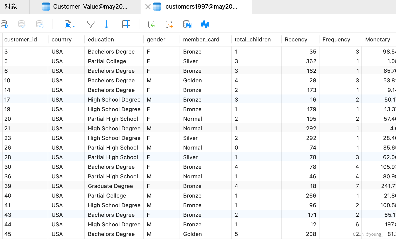
原数据如果有异常或者缺失等情况,要先对数据进行处理 ,再进行下面的操作,要不然会影响结果的正确性
一、根据RFM计算客户价值并对客户进行细分
1. 数据预处理
1.1 创建视图存储 R、F、M的最大最小值
创建视图存储R 、F、M 的最大最小值,为指标的离散提供数据
create view RFM_maxmin24(maxR,minR,maxF,minF,maxM,minM)
as
SELECT MAX(Recency) , MIN(Recency), MAX(Frequency), MIN(Frequency), MAX(Monetary), MIN(Monetary)
FROM customers1997
视图

1.2 创建视图计算对R、F、M进行离散化
注意Recency 是越小越好指标,公式同 F 和 M 有所不同
计算RFM的各项分值:
★ R ,距离当前日期越近,得分越高,最该高5分,最低1分
★ F ,交易频率越高,得分越高,最该高5分,最低1分
★ M ,交易金额越高,得分越高,最该高5分,最低1分
create view Customer_RFM
as
SELECT customer_id, Recency, Frequency, Monetary,
 CASE
   WHEN (maxR - Recency) <= (maxR - minR)/ 5 THEN 1
   WHEN (maxR - Recency) <= 2 * (maxR - minR)/ 5 THEN 2
   WHEN (maxR - Recency) <= 3 * (maxR - minR)/ 5 THEN 3
   WHEN (maxR - Recency) <= 4 * (maxR - minR)/ 5 THEN 4
   WHEN (maxR - Recency) <= 5 * (maxR - minR) / 5 THEN 5
   ELSE NULL
 END AS R,
 CASE
   WHEN (maxF - Frequency) <= (maxF - minF)/ 5 THEN 5
   WHEN (maxF - Frequency) <= 2 * (maxF - minF) / 5 THEN 4
   WHEN (maxF - Frequency) <= 3 * (maxF - minF) / 5 THEN 3
   WHEN (maxF - Frequency) <= 4 * (maxF - minF) / 5 THEN 2
   WHEN (maxF - Frequency) <= 5 * (maxF - minF) / 5 THEN 1
   ELSE NULL
 END AS F,
 CASE
   WHEN (maxM - Monetary) <= (maxM - minM) / 5 THEN 5
   WHEN (maxM - Monetary) <= 2 * (maxM - minM)/ 5 THEN 4
   WHEN (maxM - Monetary) <= 3 * (maxM - minM)/ 5 THEN 3
   WHEN (maxM - Monetary) <= 4 * (maxM - minM)/ 5 THEN 2
   WHEN (maxM - Monetary) <= 5 * (maxM - minM) / 5 THEN 1
   ELSE NULL
 END AS M
FROM customers1997 CROSS JOIN rfm_maxmin24
结果:

1.3 建立客户评分表(客户行为变量表)
CREATE TABLE Customer_Value AS
SELECT customer_id, Recency, Frequency,Monetary, R, F, M,
 R * 5 + F * 3 + M * 2 as value
FROM customer_rfm 
2. 细分客户价值
df_rfm = pd.read_csv("Customer_Value.csv") #相对路径读取数据# 客户细分
# 最佳客户(最有价值),常购客户,⼤额消费者,不确定客户(最不值钱)
# Top,High,Medium,Low
df_rfm['Segment'] = pd.cut(df_rfm['value'], 4, labels=['Low', 'Medium', 'High', 'Top'])
df_rfm
3. 创建气泡图,查看分布情况
# 创建⽓泡图
print("创建⽓泡图")
# 为不同的 Segment 分配颜⾊
color_map = {'Low': 'blue', 'Medium': 'green', 'High': 'orange', 'Top': 'red'}
colors = df_rfm['Segment'].map(color_map)
# 创建⽓泡图
plt.figure(figsize=(10, 6))
bubble_size = df_rfm['Recency'] * 5 # 调整⽓泡⼤⼩,以便更好的可视化
plt.scatter(df_rfm['Frequency'], df_rfm['Monetary'], s=bubble_size, c=colors, alpha=0.5)
plt.title('Customer Segmentation Bubble Chart')
plt.xlabel('Frequency (F)')
plt.ylabel('Monetary (M)')
plt.grid(True)
# 计算 Frequency 和 Monetary 的平均值
avg_frequency = df_rfm['Frequency'].mean()
avg_monetary = df_rfm['Monetary'].mean()
# 添加平均值参考线
plt.axvline(x=avg_frequency, color='black', linestyle='--', linewidth=1.5, label=f'Avg Frequency: {avg_frequency:.2f}')
plt.axhline(y=avg_monetary, color='black', linestyle='--', linewidth=1.5, label=f'Avg Monetary: {avg_monetary:.2f}')
# 创建图例
for segment in color_map:
 plt.scatter([], [], color=color_map[segment], label=segment, alpha=0.5, s=100)
plt.legend(title='Segment', bbox_to_anchor=(1.05, 1), loc='upper left')
plt.show()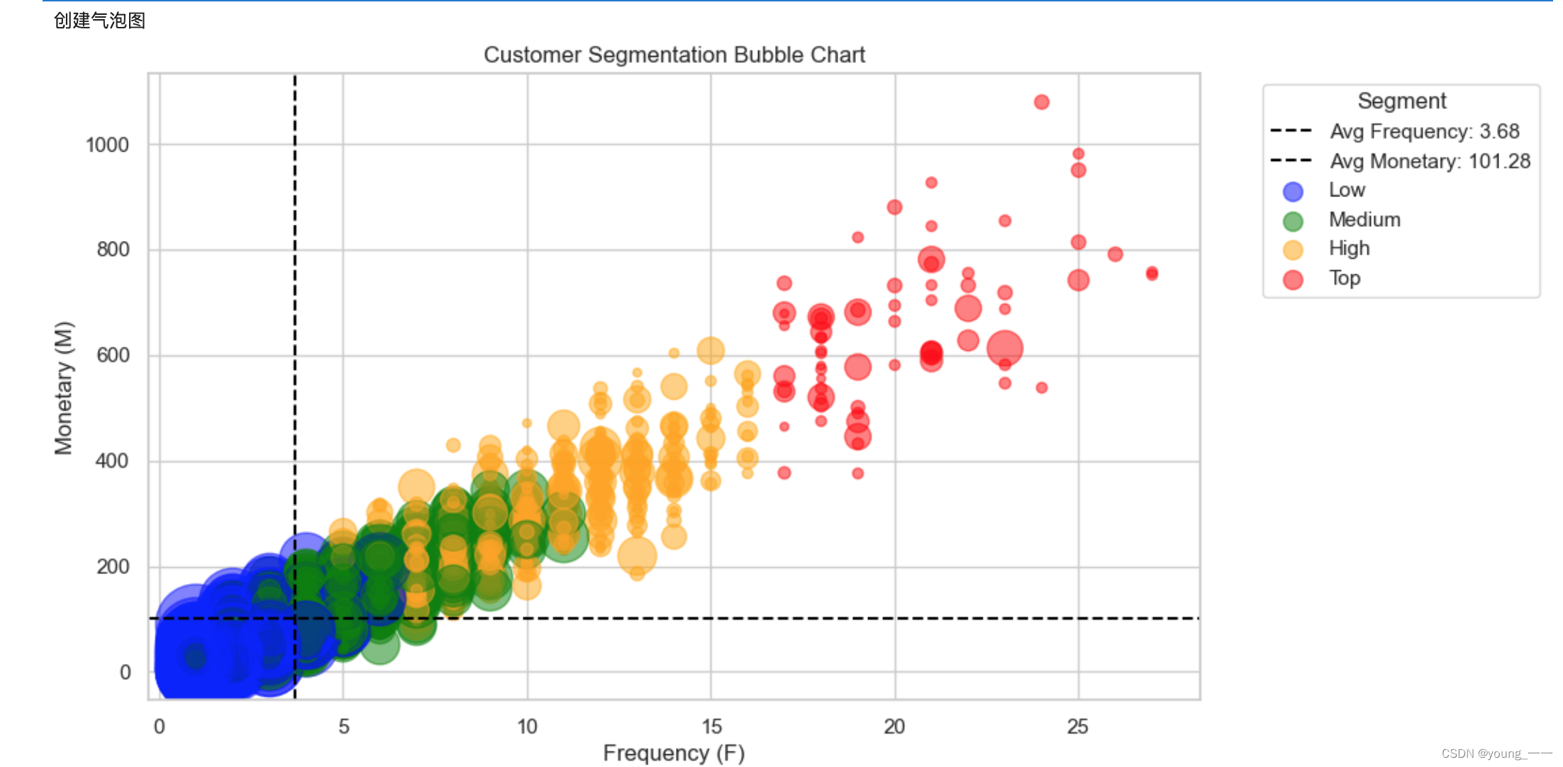
4. 分析
只分析了 top,其他方法一样
print("top用户分析")
top_customers = df_rfm[df_rfm['Segment'] == 'Top']
# 设置⻛格
sns.set(style="whitegrid")
# 创建可视化
plt.figure(figsize=(15, 5))
# Recency分布
plt.subplot(1, 3, 1)
sns.barplot(x='customer_id', y='Recency', data=top_customers, palette='cool')
plt.title('Top Customers Recency')
# Frequency分布
plt.subplot(1, 3, 2)
sns.barplot(x='customer_id', y='Frequency', data=top_customers, palette='cool')
plt.title('Top Customers Frequency')
# Monetary分布
plt.subplot(1, 3, 3)
sns.barplot(x='customer_id', y='Monetary', data=top_customers, palette='cool')
plt.title('Top Customers Monetary')
plt.tight_layout()
plt.show()
# 计算平均RFM值
avg_recency = top_customers['Recency'].mean()
avg_frequency = top_customers['Frequency'].mean()
avg_monetary = top_customers['Monetary'].mean()
# 输出结果
print(f"Top Average Recency: {avg_recency}")
print(f"Top Average Frequency: {avg_frequency}")
print(f"Top Average Monetary: {avg_monetary}")
print("top人数: ", len(top_customers)) 
5. 轮廓系数
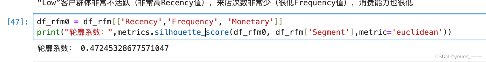
df_rfm0 = df_rfm[['Recency','Frequency', 'Monetary']]
print("轮廓系数:",metrics.silhouette_score(df_rfm0, df_rfm['Segment'],metric='euclidean'))
二、5 分法分箱(等宽/等频)对客户进行细分
分析和建模
1.“客户行为变量”表
a. 等宽
print('数据——“客户⾏为变量”表')
df #数据——“客户⾏为变量”表
# 对RFM值进⾏标准化或打分
df['R_Score'] = pd.cut(df['Recency'], 5, labels=[5, 4, 3, 2, 1])
# print(df.groupby('R_Score').R_Score.count())  # 统计各分区人数
df['F_Score'] = pd.cut(df['Frequency'], 5, labels=[1, 2, 3, 4, 5])
df['M_Score'] = pd.cut(df['Monetary'], 5, labels=[1, 2, 3, 4, 5])

# 计算RFM总分
df['RFM_Score'] = df['R_Score'].astype(int) * 5 + df['F_Score'].astype(int) * 3+ df['M_Score'].astype(int)*2
b. 等频
划分的函数qcut()和等宽的cut()不一样,其他的操作都一样
print("等频")
# 利⽤等频算法将Recency划分为5个区间
df['r_discretized_2'] = pd.qcut(r, 5, labels=range(5))
print(df.groupby('r_discretized_2').r_discretized_2.count())
2. 细分客户
# 客户细分
# 最佳客户(最有价值),常购客户,⼤额消费者,不确定客户(最不值钱)
# Top,High,Medium,Low
df['Segment'] = pd.cut(df['RFM_Score'], 4, labels=['Low', 'Medium', 'High', 'Top'])
df
3. 气泡图
# 创建⽓泡图
print("创建⽓泡图")
# 为不同的 Segment 分配颜⾊
color_map = {'Low': 'blue', 'Medium': 'green', 'High': 'orange', 'Top': 'red'}
colors = df['Segment'].map(color_map)
# 创建⽓泡图
plt.figure(figsize=(10, 6))
bubble_size = df['Recency'] * 5 # 调整⽓泡⼤⼩,以便更好的可视化
plt.scatter(df['Frequency'], df['Monetary'], s=bubble_size, c=colors, alpha=0.5)
plt.title('Customer Segmentation Bubble Chart')
plt.xlabel('Frequency (F)')
plt.ylabel('Monetary (M)')
plt.grid(True)
# 计算 Frequency 和 Monetary 的平均值
avg_frequency = df['Frequency'].mean()
avg_monetary = df['Monetary'].mean()
# 添加平均值参考线
plt.axvline(x=avg_frequency, color='black', linestyle='--', linewidth=1.5, label=f'Avg Frequency: {avg_frequency:.2f}')
plt.axhline(y=avg_monetary, color='black', linestyle='--', linewidth=1.5, label=f'Avg Monetary: {avg_monetary:.2f}')
# 创建图例
for segment in color_map:
 plt.scatter([], [], color=color_map[segment], label=segment, alpha=0.5, s=100)
plt.legend(title='Segment', bbox_to_anchor=(1.05, 1), loc='upper left')
plt.show()
4. 分析
print("top用户分析")
top_customers = df[df['Segment'] == 'Top']
# 设置⻛格
sns.set(style="whitegrid")
# 创建可视化
plt.figure(figsize=(15, 5))
# Recency分布
plt.subplot(1, 3, 1)
sns.barplot(x='customer_id', y='Recency', data=top_customers, palette='cool')
plt.title('Top Customers Recency')
# Frequency分布
plt.subplot(1, 3, 2)
sns.barplot(x='customer_id', y='Frequency', data=top_customers, palette='cool')
plt.title('Top Customers Frequency')
# Monetary分布
plt.subplot(1, 3, 3)
sns.barplot(x='customer_id', y='Monetary', data=top_customers, palette='cool')
plt.title('Top Customers Monetary')
plt.tight_layout()
plt.show()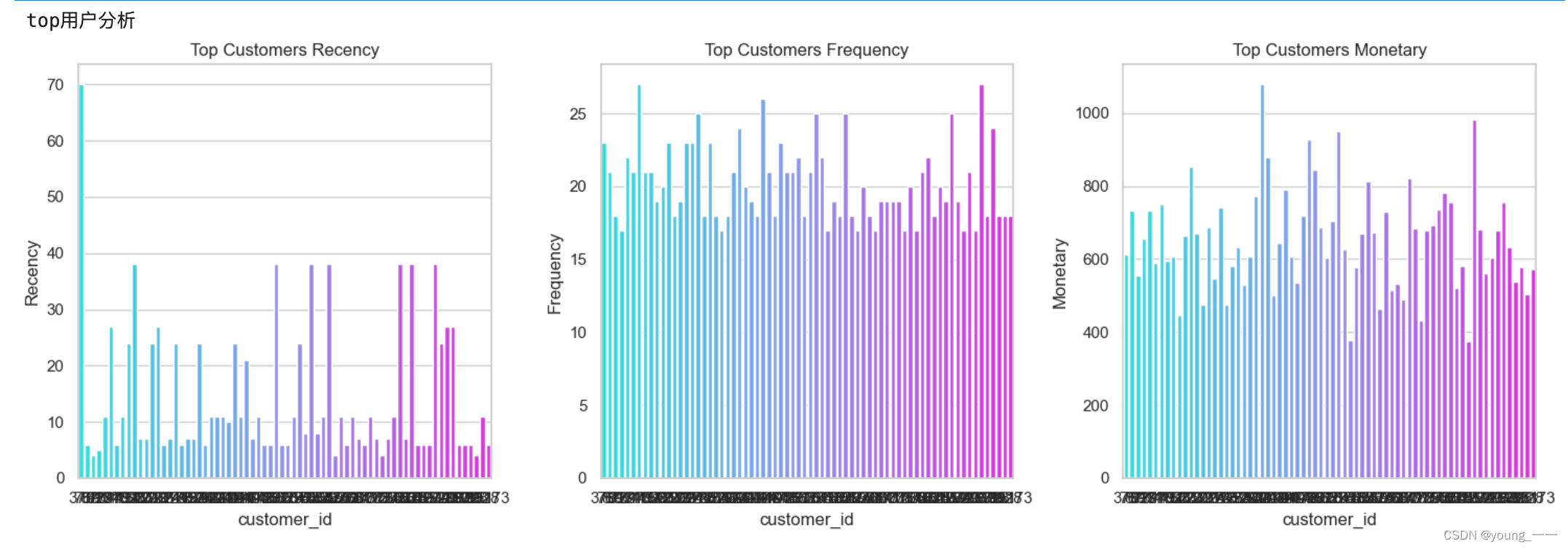
# 计算平均RFM值
avg_recency = top_customers['Recency'].mean()
avg_frequency = top_customers['Frequency'].mean()
avg_monetary = top_customers['Monetary'].mean()
# 输出结果
print(f"Top Average Recency: {avg_recency}")
print(f"Top Average Frequency: {avg_frequency}")
print(f"Top Average Monetary: {avg_monetary}")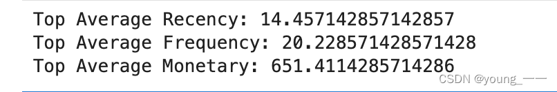
print("“Top”客户群体不仅活跃(低Recency值)⽽且⾮常忠诚(⾼Frequency值)⾼消费能⼒")
# ⼈数统计分析
education_levels = top_customers['education'].value_counts()
gender_distribution = top_customers['gender'].value_counts()
print(education_levels)
print("top人数: ")
top_counts =  len(top_customers)
print(top_counts) 
5. 轮廓系数
from sklearn import metrics
df_rfm = df[['Recency','Frequency', 'Monetary']]
print("轮廓系数:",metrics.silhouette_score(df_rfm, df['Segment'],metric='euclidean')) 
三、RFM数据标准化归一化(0-1)
import os
import pandas as pd
import numpy as np
import matplotlib.pyplot as plt
import seaborn as sns
import scipy.stats as stats
from sklearn import metrics
# pip install scikit-learn
from sklearn.preprocessing import StandardScaler, MinMaxScaler
from sklearn.impute import SimpleImputer
import warnings
warnings.filterwarnings('ignore')
%matplotlib inline
### 设置⼯作⽬录
os.chdir('/Users/mac/Documents/**/数据分析/作业/探究客户价值') #数据所在⽬录
### 数据抽取,读⼊数据
df = pd.read_csv("customers1997.csv") #相对路径读取数据
# print(df.info())
# 描述性统计
print(df.describe())常用的规范化/标准化:
数据规范化是调整数据尺度的⼀种⽅法,以便在不同的数据集之间进⾏公平⽐较。
- 最⼤-最⼩规范化:将数据缩放到0到1之间,是⼀种常⽤的归⼀化⽅法,有助于处理那些标准化假设正态分布的⽅法不适⽤的情况。
- Z分数规范化:通过数据的标准偏差来度量数据点的标准分数,有助于数据的异常值处理和去除偏差。
- ⼩数定标规范化:通过移动数据的⼩数点位置(取决于数据的最⼤绝对值)来转换数据,使得数据更加稳定和标准化。
df_fm = df[['Frequency', 'Monetary']]
# 最⼤-最⼩规范化
scaler_minmax = MinMaxScaler()
data_minmax = scaler_minmax.fit_transform(df_fm)
# Z分数规范化
scaler_standard = StandardScaler()
data_standard = scaler_standard.fit_transform(df_fm)
# ⼩数定标规范化
df_fm = df[['Frequency', 'Monetary']]
max_vals = df_fm.abs().max()
scaling_factor = np.power(10, np.ceil(np.log10(max_vals)))
df_fm_scaled = df_fm / scaling_factor

1. 数据归一化
print('将数据归一化(0-1)')
scaler_minmax = MinMaxScaler()
df_rfm = df[['Recency','Frequency', 'Monetary']]
df_rfm[['Recency','Frequency', 'Monetary']] = scaler_minmax.fit_transform(df_rfm)
print("打分")
df_rfm['R_S'] = pd.cut(df_rfm['Recency'], 5, labels=[5, 4, 3, 2, 1])
df_rfm['F_S'] = pd.cut(df_rfm['Frequency'], 5, labels=[1, 2, 3, 4, 5])
df_rfm['M_S'] = pd.cut(df_rfm['Monetary'], 5, labels=[1, 2, 3, 4, 5])
df_rfm效果:

权重根据需要填写
# 计算RFM总分
df_rfm['RFM_S'] = df_rfm['R_S'].astype(int) * 5 + df_rfm['F_S'].astype(int) * 3+ df_rfm['M_S'].astype(int)*2
2. 客户细分
# 客户细分
# 最佳客户(最有价值),常购客户,⼤额消费者,不确定客户(最不值钱)
# Top,High,Medium,Low
df_rfm['Segment'] = pd.cut(df_rfm['RFM_S'], 4, labels=['Low', 'Medium', 'High', 'Top'])
df_rfm
3. 气泡图
# 创建⽓泡图
print("创建⽓泡图")
# 为不同的 Segment 分配颜⾊
color_map = {'Low': 'blue', 'Medium': 'green', 'High': 'orange', 'Top': 'red'}
colors = df_rfm['Segment'].map(color_map)
# 创建⽓泡图
plt.figure(figsize=(10, 6))
bubble_size = df_rfm['Recency'] * 20 # 调整⽓泡⼤⼩,以便更好的可视化
plt.scatter(df_rfm['Frequency'], df_rfm['Monetary'], s=bubble_size, c=colors, alpha=0.5)
plt.title('Customer Segmentation Bubble Chart')
plt.xlabel('Frequency (F)')
plt.ylabel('Monetary (M)')
plt.grid(True)
# 计算 Frequency 和 Monetary 的平均值
avg_frequency = df_rfm['Frequency'].mean()
avg_monetary = df_rfm['Monetary'].mean()
# 添加平均值参考线
plt.axvline(x=avg_frequency, color='black', linestyle='--', linewidth=1.5, label=f'Avg Frequency: {avg_frequency:.2f}')
plt.axhline(y=avg_monetary, color='black', linestyle='--', linewidth=1.5, label=f'Avg Monetary: {avg_monetary:.2f}')
# 创建图例
for segment in color_map:
 plt.scatter([], [], color=color_map[segment], label=segment, alpha=0.5, s=100)
plt.legend(title='Segment', bbox_to_anchor=(1.05, 1), loc='upper left')
plt.show()
4.分析
print("top用户分析")
top_customers = df_rfm[df_rfm['Segment'] == 'Top']
# 计算平均RFM值
avg_recency = top_customers['Recency'].mean()
avg_frequency = top_customers['Frequency'].mean()
avg_monetary = top_customers['Monetary'].mean()
# 输出结果
print(f"Top Average Recency: {avg_recency}")
print(f"Top Average Frequency: {avg_frequency}")
print(f"Top Average Monetary: {avg_monetary}")
print("top人数: ", len(top_customers)) 
print("“Top”客户群体不仅活跃(低Recency值)⽽且⾮常忠诚(⾼Frequency值)⾼消费能⼒")5. 轮廓系数
df_rfm0 = df_rfm[['Recency','Frequency', 'Monetary']]
print("轮廓系数:",metrics.silhouette_score(df_rfm0, df_rfm['Segment'],metric='euclidean'))