目录
神经网络分类
我们以最为经典的MNIST数据集为例子,识别手写的数字(这个太经典了)
下载数据集
我们的第一步就是下载数据集完成这项任务:
%matplotlib inline
from pathlib import Path
import requests
DATA_PATH = Path("data")
PATH = DATA_PATH / "mnist"
PATH.mkdir(parents=True, exist_ok=True) # 创建一个这样的文件夹以
URL = "http://deeplearning.net/data/mnist/"
FILENAME = "mnist.pkl.gz"
if not (PATH / FILENAME).exists():
content = requests.get(URL + FILENAME).content
(PATH / FILENAME).open("wb").write(content)
1.Python绘图问题:Matplotlib中%matplotlib inline是什么、如何使用?_%matplotlib inline mial-CSDN博客,这个博客可以回答为什么整一个
%matplotlib inline我们实际上在这里做的就是将数据集写入到我们指定的包。使用的是网络包请求
下一步就是将下载的数据写入对应的地方:怎么写呢?使用Pickel模块完成这个任务:
啥是Pickle:可以简单的理解为对文件直接写入读出二进制流,省去我们操心
或者说,Pickle让数据持久化保存。pickle模块是Python专用的持久化模块,可以持久化包括自定义类在内的各种数据,比较适合Python本身复杂数据的存贮。但是持久化后的字串是不可认读的,并且只能用于Python环境,不能用作与其它语言进行数据交换。
把 Python 对象直接保存到文件里,而不需要先把它们转化为字符串再保存,也不需要用底层的文件访问操作,直接把它们写入到一个二进制文件里。pickle 模块会创建一个 Python 语言专用的二进制格式,不需要使用者考虑任何文件细节,它会帮你完成读写对象操作。用pickle比你打开文件、转换数据格式并写入这样的操作要节省不少代码行。
我们下载的是压缩的文件包(嗯,没人喜欢把数据撒拉出来一大堆),也就是说我们需要使用一个压缩包库来读取里头的数据:
import pickle import gzip with gzip.open((PATH / FILENAME).as_posix(), "rb") as f: ((x_train, y_train), (x_valid, y_valid), _) = pickle.load(f, encoding="latin-1")
加载数据集
from matplotlib import pyplot
import numpy as np
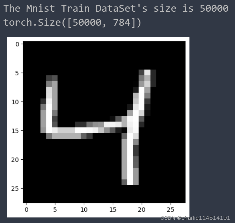
print("The Mnist Train DataSet's size is {0}".format(len(x_train)))
pyplot.imshow(x_train[2].reshape((28, 28)), cmap="gray")
print(x_train.shape)
我们上面的两行代码将x, y两个训练集的数据集加载到了程序里头。
现在,我们终于可以把目光放到使用神经网络来处理这些数据了:
实际上流程图是这样的:这个神经网络学习这些像素的排布以认识这些数字对应的像素排布是如何的,反过来做,我们就可以根据一个图像得到这个数字是什么。
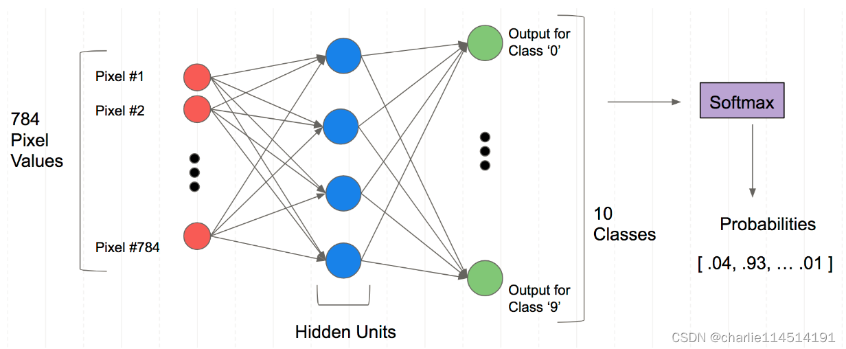
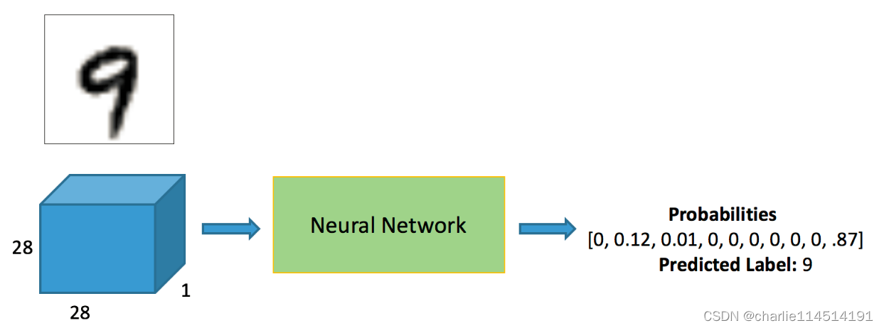
可以看到,我们的输出是一个概率图谱(也就是说:他是何种数字的概率是多少)
所以,为了转化成模型可以接受的数据格式,需要将之转化为Tensor:
import torch
x_train, y_train, x_valid, y_valid = map(
torch.tensor, (x_train, y_train, x_valid, y_valid)
)
# 下面是打印检查,可以不需要
n, c = x_train.shape
print("n= {0}, c={1}".format(n, c))
x_train, x_train.shape, y_train.min(), y_train.max()
print(x_train, y_train)
print(x_train.shape)
print(y_train.min(), y_train.max())
n= 50000, c=784
tensor([[0., 0., 0.,  ..., 0., 0., 0.],
        [0., 0., 0.,  ..., 0., 0., 0.],
        [0., 0., 0.,  ..., 0., 0., 0.],
        ...,
        [0., 0., 0.,  ..., 0., 0., 0.],
        [0., 0., 0.,  ..., 0., 0., 0.],
        [0., 0., 0.,  ..., 0., 0., 0.]]) tensor([5, 0, 4,  ..., 8, 4, 8])
torch.Size([50000, 784])
tensor(0) tensor(9)
这就是打印出来的结果。
定义损失函数
损失函数,又叫目标函数,用于计算真实值和预测值之间差异的函数,和优化器是编译一个神经网络模型的重要要素。 损失Loss必须是标量,因为向量无法比较大小(向量本身需要通过范数等标量来比较)。 损失函数一般分为4种,HingeLoss 0-1 损失函数,绝对值损失函数,平方损失函数,对数损失函数。
任何一个有负对数似然组成的损失都是定义在训练集上的经验分布和定义在模型上的概率分布之间的交叉熵。例如,均方误差是经验分布和高斯模型之间的交叉熵
这里我们两种实践方案:就是使用torch.nn.functional或者是torch.nn.Module。一般情况下,如果模型有可学习的参数,最好用nn.Module,其他情况nn.functional相对更简单一些。
所以这里,我们只是完成交叉熵损失计算,没必要上大炮:
import torch.nn.functional
loss_func = torch.nn.functional.cross_entropy
def model(xb):
    return xb.mm(weights) + bias
bs = 64 xb = x_train[0:bs] # a mini-batch from x yb = y_train[0:bs] # 生成一组随机的权重 weights = torch.randn([784, 10], dtype = torch.float, requires_grad = True) bs = 64 bias = torch.zeros(10, requires_grad=True) print(loss_func(model(xb), yb))
看看我们使用loss_func的行为如何
tensor(10.8561, grad_fn=<NllLossBackward0>)
创建模型
我们现在可以创建一个模型了:
值得注意的是:
必须继承nn.Module且在其构造函数中需调用nn.Module的构造函数
无需写反向传播函数,nn.Module能够利用autograd自动实现反向传播
Module中的可学习参数可以通过named_parameters()或者parameters()返回迭代器
from torch import nn class Mnist_NN(nn.Module): def __init__(self): # 排布好层 super().__init__() self.hidden1 = nn.Linear(784, 128) # 这里的参数说的就是输入如何,输出如何 748 -> 128 图像大小748 self.hidden2 = nn.Linear(128, 256) # 128 -> 256 self.out = nn.Linear(256, 10) # 256 -> 10 结果是10个 def forward(self, x): # 向前推理的函数 x = F.relu(self.hidden1(x)) x = F.relu(self.hidden2(x)) x = self.out(x) return x
net = Mnist_NN() # 实例化一个网络出来
print(net)
可以看看结果:
hidden1.weight Parameter containing:
tensor([[ 0.0352,  0.0222,  0.0229,  ..., -0.0060, -0.0189, -0.0097],
        [-0.0067,  0.0222, -0.0206,  ..., -0.0217,  0.0225,  0.0059],
        [ 0.0255, -0.0330,  0.0099,  ...,  0.0030, -0.0336, -0.0115],
        ...,
        [ 0.0060,  0.0357,  0.0064,  ..., -0.0156,  0.0180,  0.0014],
        [-0.0235,  0.0185,  0.0324,  ...,  0.0238,  0.0045, -0.0037],
        [ 0.0342,  0.0153,  0.0076,  ..., -0.0325, -0.0033, -0.0302]],
       requires_grad=True) torch.Size([128, 784])
hidden1.bias Parameter containing:
tensor([ 0.0089, -0.0122, -0.0346,  0.0320, -0.0041, -0.0223, -0.0190,  0.0334,
        -0.0238,  0.0318, -0.0080, -0.0203,  0.0054,  0.0291, -0.0009, -0.0321,
         0.0285,  0.0037,  0.0058, -0.0081, -0.0128,  0.0249,  0.0216, -0.0272,
         0.0097,  0.0126, -0.0058, -0.0149,  0.0192,  0.0115, -0.0009, -0.0009,
         0.0065, -0.0151,  0.0241,  0.0203,  0.0239, -0.0265, -0.0227,  0.0166,
         0.0351, -0.0198, -0.0105, -0.0181,  0.0059, -0.0214,  0.0196,  0.0210,
        -0.0053, -0.0342, -0.0183, -0.0230, -0.0006, -0.0349,  0.0306,  0.0018,
        -0.0130,  0.0113,  0.0059, -0.0110,  0.0043,  0.0049,  0.0171,  0.0256,
        -0.0287, -0.0170, -0.0231,  0.0072, -0.0046, -0.0164,  0.0252, -0.0138,
        -0.0206, -0.0213, -0.0110, -0.0056, -0.0336,  0.0229, -0.0170, -0.0048,
         0.0185, -0.0346,  0.0248,  0.0061, -0.0257,  0.0040, -0.0019, -0.0145,
        -0.0328,  0.0062,  0.0053, -0.0172, -0.0061, -0.0245, -0.0230,  0.0222,
         0.0216,  0.0206,  0.0062, -0.0151, -0.0266,  0.0320, -0.0082,  0.0160,
         0.0224,  0.0243,  0.0039,  0.0010,  0.0316,  0.0178,  0.0290,  0.0259,
         0.0215, -0.0204, -0.0100,  0.0303,  0.0062,  0.0035,  0.0245, -0.0189,
...
       requires_grad=True) torch.Size([10, 256])
out.bias Parameter containing:
tensor([-0.0375,  0.0110, -0.0267, -0.0310,  0.0062,  0.0310,  0.0617, -0.0109,
         0.0520,  0.0088], requires_grad=True) torch.Size([10])
使用DataSet和DataLoader化简我们的数据封装
from torch.utils.data import TensorDataset from torch.utils.data import DataLoader train_ds = TensorDataset(x_train, y_train) train_dl = DataLoader(train_ds, batch_size=bs, shuffle=True) valid_ds = TensorDataset(x_valid, y_valid) valid_dl = DataLoader(valid_ds, batch_size=bs * 2) def get_data(train_ds, valid_ds, bs): return ( DataLoader(train_ds, batch_size=bs, shuffle=True), DataLoader(valid_ds, batch_size=bs * 2), )
我们将数据封装成稍后函数将会用到的格式,如上👆
import numpy as np
# 下面定义拟合函数,这里实际上就是我们的训练应用层!
# Steps: 训练的论数
# loss_func: 我们之前定义的损失函数
# opt: 这里我们指代的是优化算子方法,比如说,我们这里使用SGD
# train_dl: 训练的数据集
# valid_dl: 验证的数据集
def fit(steps, model, loss_func, opt, train_dl, valid_dl):
for step in range(steps):
model.train()
for xb, yb in train_dl:
loss_batch(model, loss_func, xb, yb, opt)
model.eval()
with torch.no_grad():
losses, nums = zip(
*[loss_batch(model, loss_func, xb, yb) for xb, yb in valid_dl]
)
val_loss = np.sum(np.multiply(losses, nums)) / np.sum(nums)
print('当前step:'+str(step), '验证集损失:'+str(val_loss))
一般在训练模型时加上model.train(),这样会正常使用Batch Normalization和 Dropout
测试的时候一般选择model.eval(),这样就不会使用Batch Normalization和 Dropout
下面,我们终于可以开始进行数据集训练了:
train_dl, valid_dl = get_data(train_ds, valid_ds, bs)
model, opt = get_model()
fit(30, model, loss_func, opt, train_dl, valid_dl)
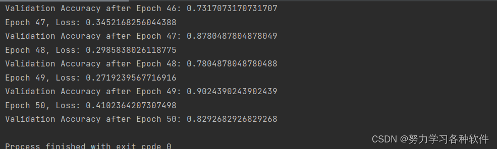
看看结果!
当前step:0 验证集损失:2.273305953979492
当前step:1 验证集损失:2.237687868499756
当前step:2 验证集损失:2.1822078701019287
当前step:3 验证集损失:2.0902939651489256
当前step:4 验证集损失:1.9395794193267821
当前step:5 验证集损失:1.7149433799743652
当前step:6 验证集损失:1.4407895727157594
当前step:7 验证集损失:1.1795400686264037
当前step:8 验证集损失:0.9769629907608032
当前step:9 验证集损失:0.8321391986846924
当前step:10 验证集损失:0.7286654480934143
当前step:11 验证集损失:0.6524578206062317
当前step:12 验证集损失:0.5956221778869629
当前step:13 验证集损失:0.5517672945976257
当前step:14 验证集损失:0.5173421884059906
当前step:15 验证集损失:0.48939590430259705
当前step:16 验证集损失:0.4668446585178375
当前step:17 验证集损失:0.4478798774242401
当前step:18 验证集损失:0.43193086733818054
当前step:19 验证集损失:0.4181952142238617
当前step:20 验证集损失:0.40629616613388064
当前step:21 验证集损失:0.396016849565506
当前step:22 验证集损失:0.38692939014434813
当前step:23 验证集损失:0.3788792317867279
当前step:24 验证集损失:0.3714227032661438
当前step:25 验证集损失:0.36518091886043547
当前step:26 验证集损失:0.3593594216585159
当前step:27 验证集损失:0.3533795116186142
当前step:28 验证集损失:0.34808647682666777
当前step:29 验证集损失:0.3436836592435837
使用Pytorch神经网络进行气温预测
使用到的包:
import numpy as np
import pandas as pd
import matplotlib.pyplot as plt
import torch
import torch.optim as optim
import warnings
warnings.filterwarnings("ignore")
%matplotlib inline
features = pd.read_csv('temps.csv')
#看看数据长什么样子
features.head()
# 如果想要调整,可以输入一个数组指定查看若干行
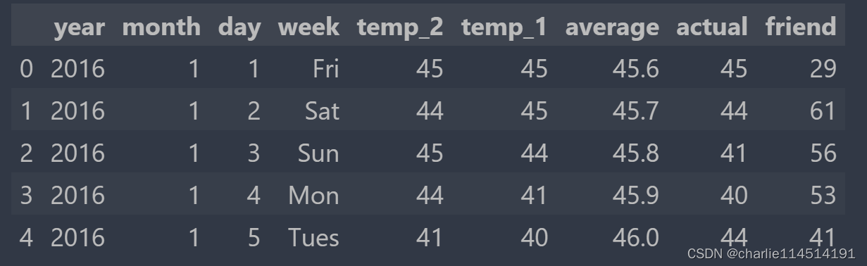
数据表中
* year,moth,day,week分别表示的具体的时间
* temp_2:前天的最高温度值
* temp_1:昨天的最高温度值
* average:在历史中,每年这一天的平均最高温度值
* actual:这就是我们的标签值了,当天的真实最高温度
* friend:这一列可能是凑热闹的,你的朋友猜测的可能值,咱们不管它就好了
我想说的是:这跟我们实际收集到的数据一样,可能会存在一些垃圾值需要我们的处理!
# 处理时间数据 import datetime # 分别得到年,月,日 years = features['year'] months = features['month'] days = features['day'] # datetime格式 dates = [str(int(year)) + '-' + str(int(month)) + '-' + str(int(day)) for year, month, day in zip(years, months, days)] dates = [datetime.datetime.strptime(date, '%Y-%m-%d') for date in dates] dates[:5]
[datetime.datetime(2016, 1, 1, 0, 0),
 datetime.datetime(2016, 1, 2, 0, 0),
 datetime.datetime(2016, 1, 3, 0, 0),
 datetime.datetime(2016, 1, 4, 0, 0),
 datetime.datetime(2016, 1, 5, 0, 0)]
我们来画图看看:
# 准备画图
# 指定默认风格
plt.style.use('fivethirtyeight')
# 设置布局
fig, ((ax1, ax2), (ax3, ax4)) = plt.subplots(nrows=2, ncols=2, figsize = (10,10))
fig.autofmt_xdate(rotation = 45)
# 标签值
ax1.plot(dates, features['actual'])
ax1.set_xlabel(''); ax1.set_ylabel('Temperature'); ax1.set_title('Max Temp')
# 昨天
ax2.plot(dates, features['temp_1'])
ax2.set_xlabel(''); ax2.set_ylabel('Temperature'); ax2.set_title('Previous Max Temp')
# 前天
ax3.plot(dates, features['temp_2'])
ax3.set_xlabel('Date'); ax3.set_ylabel('Temperature'); ax3.set_title('Two Days Prior Max Temp')
# 我的逗逼朋友
ax4.plot(dates, features['friend'])
ax4.set_xlabel('Date'); ax4.set_ylabel('Temperature'); ax4.set_title('Friend Estimate')
plt.tight_layout(pad=2)
下面,我们进一步处理数据的标签问题:可以看到我们的属性还是字符串,我们如何将之映射为网络可以理解的结构呢:使用独热编码:
在很多机器学习任务中,特征并不总是连续值,而有可能是分类值。
离散特征的编码分为两种情况:
离散特征的取值之间没有大小的意义,比如color:[red,blue],那么就使用one-hot编码
离散特征的取值有大小的意义,比如size:[X,XL,XXL],那么就使用数值的映射{X:1,XL:2,XXL:3}
# 标签
labels = np.array(features['actual'])
# 在特征中去掉标签
features= features.drop('actual', axis = 1)
# 名字单独保存一下,以备后患
feature_list = list(features.columns)
# 转换成合适的格式
features = np.array(features)
这个时候我们会发现,这些特征的量级大小不一,会很容易造成偏置,一个办法就是对之进行正则化:
from sklearn import preprocessing
# 使用标准化来处理数据
# fit后变化
input_features = preprocessing.StandardScaler().fit_transform(features)
# 看看结果:
input_features[0]
array([ 0.        , -1.5678393 , -1.65682171, -1.48452388, -1.49443549,
       -1.3470703 , -1.98891668,  2.44131112, -0.40482045, -0.40961596,
       -0.40482045, -0.40482045, -0.41913682, -0.40482045])
构建网络模型
两种方式:一种我们手动来:
x = torch.tensor(input_features, dtype = float)
y = torch.tensor(labels, dtype = float)
# 权重参数初始化
weights = torch.randn((14, 128), dtype = float, requires_grad = True)
biases = torch.randn(128, dtype = float, requires_grad = True)
weights2 = torch.randn((128, 1), dtype = float, requires_grad = True)
biases2 = torch.randn(1, dtype = float, requires_grad = True)
learning_rate = 0.001
losses = []
for i in range(1000):
# 计算隐层
hidden = x.mm(weights) + biases
# 加入激活函数
hidden = torch.relu(hidden)
# 预测结果
predictions = hidden.mm(weights2) + biases2
# 通计算损失
loss = torch.mean((predictions - y) ** 2)
losses.append(loss.data.numpy())
# 打印损失值
if i % 100 == 0:
print('loss:', loss)
#返向传播计算
loss.backward()
#更新参数
weights.data.add_(- learning_rate * weights.grad.data)
biases.data.add_(- learning_rate * biases.grad.data)
weights2.data.add_(- learning_rate * weights2.grad.data)
biases2.data.add_(- learning_rate * biases2.grad.data)
# 每次迭代都得记得清空
weights.grad.data.zero_()
biases.grad.data.zero_()
weights2.grad.data.zero_()
biases2.grad.data.zero_()
loss: tensor(4447.1342, dtype=torch.float64, grad_fn=<MeanBackward0>)
loss: tensor(157.0553, dtype=torch.float64, grad_fn=<MeanBackward0>)
loss: tensor(148.6876, dtype=torch.float64, grad_fn=<MeanBackward0>)
loss: tensor(145.6146, dtype=torch.float64, grad_fn=<MeanBackward0>)
loss: tensor(143.9219, dtype=torch.float64, grad_fn=<MeanBackward0>)
loss: tensor(142.8372, dtype=torch.float64, grad_fn=<MeanBackward0>)
loss: tensor(142.0914, dtype=torch.float64, grad_fn=<MeanBackward0>)
loss: tensor(141.5533, dtype=torch.float64, grad_fn=<MeanBackward0>)
loss: tensor(141.1492, dtype=torch.float64, grad_fn=<MeanBackward0>)
loss: tensor(140.8404, dtype=torch.float64, grad_fn=<MeanBackward0>)
另一种用库:
input_size = input_features.shape[1]
hidden_size = 128
output_size = 1
batch_size = 16
my_nn = torch.nn.Sequential(
    torch.nn.Linear(input_size, hidden_size),
    torch.nn.Sigmoid(),
    torch.nn.Linear(hidden_size, output_size),
)
cost = torch.nn.MSELoss(reduction='mean')
optimizer = torch.optim.Adam(my_nn.parameters(), lr = 0.001)
# 训练网络
losses = []
for i in range(1000):
    batch_loss = []
    # MINI-Batch方法来进行训练
    for start in range(0, len(input_features), batch_size):
        end = start + batch_size if start + batch_size < len(input_features) else len(input_features)
        xx = torch.tensor(input_features[start:end], dtype = torch.float, requires_grad = True)
        yy = torch.tensor(labels[start:end], dtype = torch.float, requires_grad = True)
        prediction = my_nn(xx)
        loss = cost(prediction, yy)
        optimizer.zero_grad()
        loss.backward(retain_graph=True)
        optimizer.step()
        batch_loss.append(loss.data.numpy())

    # 打印损失
    if i % 100==0:
        losses.append(np.mean(batch_loss))
        print(i, np.mean(batch_loss))
我们取出结果:
x = torch.tensor(input_features, dtype = torch.float)
predict = my_nn(x).data.numpy()
值得注意的是:我们的验证集也需要按照相同的方式进行预处理后才可以放到模型里预测:
# 转换日期格式
dates = [str(int(year)) + '-' + str(int(month)) + '-' + str(int(day)) for year, month, day in zip(years, months, days)]
dates = [datetime.datetime.strptime(date, '%Y-%m-%d') for date in dates]
# 创建一个表格来存日期和其对应的标签数值
true_data = pd.DataFrame(data = {'date': dates, 'actual': labels})
# 同理,再创建一个来存日期和其对应的模型预测值
months = features[:, feature_list.index('month')]
days = features[:, feature_list.index('day')]
years = features[:, feature_list.index('year')]
test_dates = [str(int(year)) + '-' + str(int(month)) + '-' + str(int(day)) for year, month, day in zip(years, months, days)]
test_dates = [datetime.datetime.strptime(date, '%Y-%m-%d') for date in test_dates]
predictions_data = pd.DataFrame(data = {'date': test_dates, 'prediction': predict.reshape(-1)})
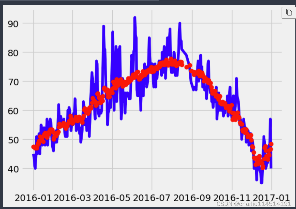
# 真实值
plt.plot(true_data['date'], true_data['actual'], 'b-', label = 'actual')
# 预测值
plt.plot(predictions_data['date'], predictions_data['prediction'], 'ro', label = 'prediction')
plt.xticks(rotation = '60');
plt.legend()
# 图名
plt.xlabel('Date'); plt.ylabel('Maximum Temperature (F)'); plt.title('Actual and Predicted Values');
Reference
Python绘图问题:Matplotlib中%matplotlib inline是什么、如何使用?_%matplotlib inline mial-CSDN博客
一文带你搞懂Python中pickle模块 - 知乎 (zhihu.com)


![[docker] 镜像部分补充](https://img-blog.csdnimg.cn/direct/94e3babe7a6c48a3b46967cd8f73f014.png)