import os
os.environ['TF_CPP_MIN_LOG_LEVEL'] = '2'#设置tensorflow的日志级别
from tensorflow.python.platform import build_info
import tensorflow as tf
# 列出所有物理GPU设备
gpus = tf.config.list_physical_devices('GPU')
if gpus:
# 如果有GPU,设置GPU资源使用率
try:
# 允许GPU内存按需增长
for gpu in gpus:
tf.config.experimental.set_memory_growth(gpu, True)
# 设置可见的GPU设备(这里实际上不需要,因为已经通过内存增长设置了每个GPU)
# tf.config.set_visible_devices(gpus, 'GPU')
print("GPU可用并已设置内存增长模式。")
except RuntimeError as e:
# 虚拟设备未就绪时可能无法设置GPU
print(f"设置GPU时发生错误: {e}")
else:
# 如果没有GPU
print("没有检测到GPU设备。")
import numpy as np
import matplotlib.pyplot as plt
print(tf.__version__)
fashion_mnist = tf.keras.datasets.fashion_mnist
(train_images, train_labels), (test_images, test_labels) = fashion_mnist.load_data()
# 将数据保存到 npz 文件中
np.savez_compressed('./datasets/fashion_mnist.npz',
train_images=train_images,
train_labels=train_labels,
test_images=test_images,
test_labels=test_labels)
data=np.load('./datasets/fashion_mnist.npz')
train_images = data['train_images']
train_labels = data['train_labels']
test_images = data['test_images']
test_labels = data['test_labels']
print(train_images.shape,train_labels.shape,np.unique(train_labels))
print(train_images.max(),train_images.min())
#数字标签对应的类别
class_names = ['T-shirt/top', 'Trouser', 'Pullover', 'Dress', 'Coat',
'Sandal', 'Shirt', 'Sneaker', 'Bag', 'Ankle boot']
plt.figure()
plt.imshow(train_images[0])
plt.colorbar()
plt.grid(False)
plt.show()
# 将这些值缩小至 0 到 1 之间,然后将其馈送到神经网络模型
#归一化
train_images = train_images / 255.0
test_images = test_images / 255.0
plt.figure(figsize=(10,10))
for i in range(25):#展示25张图片
plt.subplot(5,5,i+1)#以子视图的形式展示
plt.xticks([])#不带刻度
plt.yticks([])
plt.grid(False) #不带网格
plt.imshow(train_images[i], cmap=plt.cm.binary)
plt.xlabel(class_names[train_labels[i]])#显示横轴标签为数字标签对应的真实类别
plt.show()
model = tf.keras.Sequential([
tf.keras.layers.Input(shape=((28,28))),
tf.keras.layers.Flatten(),#扁平化处理成行向量
tf.keras.layers.Dense(128, activation='relu'),#线性转换层
tf.keras.layers.Dense(10)#输出层,10个分值,对应模型对于输入数据应该属于这10个类别的置信度
])
model.summary()
#优化器,损失函数,指标,这个损失会对标签做类似one-hot的处理
model.compile(optimizer='adam',
loss=tf.keras.losses.SparseCategoricalCrossentropy(from_logits=True),
metrics=['accuracy'])
model.fit(train_images, train_labels, epochs=10)
test_loss, test_acc = model.evaluate(test_images, test_labels, verbose=2)
print('\nTest accuracy:', test_acc)
#模型训练好后可以加一个概率层把logits转换成概率
probability_model = tf.keras.Sequential([model,
tf.keras.layers.Softmax()])
predictions = probability_model.predict(test_images)
np.argmax(predictions[0])#获取其中最大值对应的索引下标
test_labels[0]
def plot_image(i, predictions_array, true_label, img):
true_label, img = true_label[i], img[i]
plt.grid(False)
plt.xticks([])
plt.yticks([])
plt.imshow(img, cmap=plt.cm.binary)
predicted_label = np.argmax(predictions_array)
if predicted_label == true_label:
color = 'blue'
else:
color = 'red'
plt.xlabel("{} {:2.0f}% ({})".format(class_names[predicted_label],
100*np.max(predictions_array),
class_names[true_label]),
color=color)
def plot_value_array(i, predictions_array, true_label):
true_label = true_label[i]
plt.grid(False)
plt.xticks(range(10))
plt.yticks([])
thisplot = plt.bar(range(10), predictions_array, color="#777777")
plt.ylim([0, 1])
predicted_label = np.argmax(predictions_array)
thisplot[predicted_label].set_color('red')
thisplot[true_label].set_color('blue')
i = 0
plt.figure(figsize=(6,3))
plt.subplot(1,2,1)
plot_image(i, predictions[i], test_labels, test_images)
plt.subplot(1,2,2)
plot_value_array(i, predictions[i], test_labels)
plt.show()
i = 12
plt.figure(figsize=(6,3))
plt.subplot(1,2,1)
plot_image(i, predictions[i], test_labels, test_images)
plt.subplot(1,2,2)
plot_value_array(i, predictions[i], test_labels)
plt.show()
# 让我们用模型的预测绘制几张图像。请注意,即使置信度很高,模型也可能出错
num_rows = 5
num_cols = 3
num_images = num_rows*num_cols
plt.figure(figsize=(2*2*num_cols, 2*num_rows))
for i in range(num_images):
plt.subplot(num_rows, 2*num_cols, 2*i+1)
plot_image(i, predictions[i], test_labels, test_images)
plt.subplot(num_rows, 2*num_cols, 2*i+2)
plot_value_array(i, predictions[i], test_labels)
plt.tight_layout()
plt.show()
#最后,使用训练好的模型对单个图像进行预测
img = test_images[1]
print(img.shape)
#在0轴增加1个维度
img = (np.expand_dims(img,0))
print(img.shape)
predictions_single = probability_model.predict(img)
print(predictions_single)
plot_value_array(1, predictions_single[0], test_labels)
_ = plt.xticks(range(10), class_names, rotation=45)
plt.show()
np.argmax(predictions_single[0])
test_labels[1]