本文为此系列的第四篇conditional GAN,上一篇为WGAN-GP。文中在无监督的基础上重点讲解作为有监督对比无监督的差异,若有不懂的无监督知识点可以看本系列第一篇。
原理
有条件与无条件

如图投进硬币随机得到一个乒乓球的例子可以看成是一个无监督的GAN,硬币作为输入(noise),出乒乓球的机器作为生成器(generator),生成的乒乓球作为生成器生成的example。
从这个例子中我们可以知道生成的乒乓球有什么颜色的,因为这些都是我们训练的数据分布,但我们不知道生成的是什么颜色的乒乓球,因为是无监督的。

这个例子中,投掷硬币和输入想要的饮料名称例如红色的苏打水,就会随机投出一瓶选定类型的红色苏打水,而不会投出绿色的雪碧。
这里不同于上面的例子的是输入中多了一个饮料名称(class),以及输出可以选择想要的类型。这里输入的类别必须在机器给定的类别之内选择不能选择没有给定的类别,就好像我们训练时只训练这些类别生成器就只知道这些类别的东西,其他类别的东西就会出错。
这样可以选择类别输出的例子就是有监督的。注意:这里虽然可以选择类别输出,但不能控制特性输出,比如我们可以选择投出一瓶苏打水,但不能选择固定生产日期的苏打水,或者某品牌的苏打水等,这类可控制特性输出的叫做Controllable
GAN,在下一篇作讲解。
这就是有条件与无条件的区别,有条件的在训练时数据需要有标签,前向传播时输入生成器还需要多加一个class向量。
输入

如图,在无监督的GAN中,噪声向量也是一维的;在有监督中的GAN中,我们所需的class也要是one-hot形式的一维向量(长度为类别数量)。但我们不是直接将两个向量输入进生成器中,而是合成一个向量。

作为generator的输入如图:

输入进discriminator也是需要有class的信息


但是不是想上图这样分开作为两个向量的输入,而是也是合成为一个向量进行输入。但是图像信息作为三维向量,类别信息作为一维向量,就需要进行处理:

类别信息要先转为one-hot形式,然后每个类别处理成一个image_height * image_width的二维向量作为一个channel与图像信息进行concat。
代码
model.py
from torch import nn

class Generator(nn.Module):
    def __init__(self, input_dim=10, im_chan=1, hidden_dim=64):
        super(Generator, self).__init__()
        self.input_dim = input_dim
        # Build the neural network
        self.gen = nn.Sequential(
            self.make_gen_block(input_dim, hidden_dim * 4),
            self.make_gen_block(hidden_dim * 4, hidden_dim * 2, kernel_size=4, stride=1),
            self.make_gen_block(hidden_dim * 2, hidden_dim),
            self.make_gen_block(hidden_dim, im_chan, kernel_size=4, final_layer=True),
        )

    def make_gen_block(self, input_channels, output_channels, kernel_size=3, stride=2, final_layer=False):
        if not final_layer:
            return nn.Sequential(
                nn.ConvTranspose2d(input_channels, output_channels, kernel_size, stride),
                nn.BatchNorm2d(output_channels),
                nn.ReLU(inplace=True),
            )
        else:
            return nn.Sequential(
                nn.ConvTranspose2d(input_channels, output_channels, kernel_size, stride),
                nn.Tanh(),
            )

    def forward(self, noise):
        x = noise.view(len(noise), self.input_dim, 1, 1)
        return self.gen(x)

class Discriminator(nn.Module):
    def __init__(self, im_chan=1, hidden_dim=64):
        super(Discriminator, self).__init__()
        self.disc = nn.Sequential(
            self.make_disc_block(im_chan, hidden_dim),
            self.make_disc_block(hidden_dim, hidden_dim * 2),
            self.make_disc_block(hidden_dim * 2, 1, final_layer=True),
        )

    def make_disc_block(self, input_channels, output_channels, kernel_size=4, stride=2, final_layer=False):
        if not final_layer:
            return nn.Sequential(
                nn.Conv2d(input_channels, output_channels, kernel_size, stride),
                nn.BatchNorm2d(output_channels),
                nn.LeakyReLU(0.2, inplace=True),
            )
        else:
            return nn.Sequential(
                nn.Conv2d(input_channels, output_channels, kernel_size, stride),
            )

    def forward(self, image):
        disc_pred = self.disc(image)
        return disc_pred.view(len(disc_pred), -1)
train.py
import torch
from torch import nn
from tqdm.auto import tqdm
from torchvision import transforms
from torchvision.datasets import MNIST
from torchvision.utils import make_grid
from torch.utils.data import DataLoader
import torch.nn.functional as F
import matplotlib.pyplot as plt
from model import *
torch.manual_seed(0) # Set for our testing purposes, please do not change!

def show_tensor_images(image_tensor, num_images=25, size=(1, 28, 28), nrow=5, show=True):
    '''
    Function for visualizing images: Given a tensor of images, number of images, and
    size per image, plots and prints the images in an uniform grid.
    '''
    image_tensor = (image_tensor + 1) / 2
    image_unflat = image_tensor.detach().cpu()
    image_grid = make_grid(image_unflat[:num_images], nrow=nrow)
    plt.imshow(image_grid.permute(1, 2, 0).squeeze())
    if show:
        plt.show()

def get_noise(n_samples, input_dim, device='cpu'):
    '''
    Function for creating noise vectors: Given the dimensions (n_samples, input_dim)
    creates a tensor of that shape filled with random numbers from the normal distribution.
    Parameters:
        n_samples: the number of samples to generate, a scalar
        input_dim: the dimension of the input vector, a scalar
        device: the device type
    '''
    return torch.randn(n_samples, input_dim, device=device)

def get_one_hot_labels(labels, n_classes):
    return F.one_hot(labels,n_classes)

def combine_vectors(x, y):
    combined = torch.cat((x.float(),y.float()), 1)
    return combined

mnist_shape = (1, 28, 28)
n_classes = 10

criterion = nn.BCEWithLogitsLoss()
n_epochs = 200
z_dim = 64
display_step = 500
batch_size = 128
lr = 0.0002
device = 'cuda'

transform = transforms.Compose([
    transforms.ToTensor(),
    transforms.Normalize((0.5,), (0.5,)),
])

dataloader = DataLoader(
    MNIST('.', download=False, transform=transform),
    batch_size=batch_size,
    shuffle=True)

def get_input_dimensions(z_dim, mnist_shape, n_classes):
    generator_input_dim = z_dim + n_classes
    discriminator_im_chan = mnist_shape[0] + n_classes
    return generator_input_dim, discriminator_im_chan

generator_input_dim, discriminator_im_chan = get_input_dimensions(z_dim, mnist_shape, n_classes)

gen = Generator(input_dim=generator_input_dim).to(device)
gen_opt = torch.optim.Adam(gen.parameters(), lr=lr)
disc = Discriminator(im_chan=discriminator_im_chan).to(device)
disc_opt = torch.optim.Adam(disc.parameters(), lr=lr)

def weights_init(m):
    if isinstance(m, nn.Conv2d) or isinstance(m, nn.ConvTranspose2d):
        torch.nn.init.normal_(m.weight, 0.0, 0.02)
    if isinstance(m, nn.BatchNorm2d):
        torch.nn.init.normal_(m.weight, 0.0, 0.02)
        torch.nn.init.constant_(m.bias, 0)
gen = gen.apply(weights_init)
disc = disc.apply(weights_init)

cur_step = 0
generator_losses = []
discriminator_losses = []

# UNIT TEST NOTE: Initializations needed for grading
noise_and_labels = False
fake = False

fake_image_and_labels = False
real_image_and_labels = False
disc_fake_pred = False
disc_real_pred = False

best_gen_loss = float('inf')
last_gen_loss = 0

for epoch in range(n_epochs):
    # Dataloader returns the batches and the labels
    for real, labels in tqdm(dataloader):
        cur_batch_size = len(real)
        # Flatten the batch of real images from the dataset
        real = real.to(device)

        one_hot_labels = get_one_hot_labels(labels.to(device), n_classes)
        image_one_hot_labels = one_hot_labels[:, :, None, None]
        image_one_hot_labels = image_one_hot_labels.repeat(1, 1, mnist_shape[1], mnist_shape[2])

        ### Update discriminator ###
        # Zero out the discriminator gradients
        disc_opt.zero_grad()
        # Get noise corresponding to the current batch_size
        fake_noise = get_noise(cur_batch_size, z_dim, device=device)

        noise_and_labels = combine_vectors(fake_noise, one_hot_labels)
        fake = gen(noise_and_labels)

        fake_image_and_labels = combine_vectors(fake, image_one_hot_labels)
        real_image_and_labels = combine_vectors(real, image_one_hot_labels)
        disc_fake_pred = disc(fake_image_and_labels.detach())
        disc_real_pred = disc(real_image_and_labels)

        disc_fake_loss = criterion(disc_fake_pred, torch.zeros_like(disc_fake_pred))
        disc_real_loss = criterion(disc_real_pred, torch.ones_like(disc_real_pred))
        disc_loss = (disc_fake_loss + disc_real_loss) / 2
        disc_loss.backward(retain_graph=True)
        disc_opt.step()

        # Keep track of the average discriminator loss
        discriminator_losses += [disc_loss.item()]

        ### Update generator ###
        # Zero out the generator gradients
        gen_opt.zero_grad()

        fake_image_and_labels = combine_vectors(fake, image_one_hot_labels)
        # This will error if you didn't concatenate your labels to your image correctly
        disc_fake_pred = disc(fake_image_and_labels)
        gen_loss = criterion(disc_fake_pred, torch.ones_like(disc_fake_pred))
        gen_loss.backward()
        gen_opt.step()

        # Keep track of the generator losses
        generator_losses += [gen_loss.item()]

        if cur_step % display_step == 0 and cur_step > 0:
            gen_mean = sum(generator_losses[-display_step:]) / display_step
            disc_mean = sum(discriminator_losses[-display_step:]) / display_step
            print(f"Step {cur_step}: Generator loss: {gen_mean}, discriminator loss: {disc_mean}")
            show_tensor_images(fake)
            show_tensor_images(real)
            step_bins = 20
            x_axis = sorted([i * step_bins for i in range(len(generator_losses) // step_bins)] * step_bins)
            num_examples = (len(generator_losses) // step_bins) * step_bins
            plt.plot(
                range(num_examples // step_bins),
                torch.Tensor(generator_losses[:num_examples]).view(-1, step_bins).mean(1),
                label="Generator Loss"
            )
            plt.plot(
                range(num_examples // step_bins),
                torch.Tensor(discriminator_losses[:num_examples]).view(-1, step_bins).mean(1),
                label="Discriminator Loss"
            )
            plt.legend()
            plt.show()
        elif cur_step == 0:
            print(
                "Congratulations! If you've gotten here, it's working. Please let this train until you're happy with how the generated numbers look, and then go on to the exploration!")
        cur_step += 1

        # Save generator model
        if gen_loss < best_gen_loss:
            best_gen_loss = gen_loss
            torch.save(gen.state_dict(), 'best_generator.pth')
        last_gen_loss = gen_loss
        torch.save(gen.state_dict(), 'last_generator.pth')


# test
import math
gen = gen.eval()

checkpoint = torch.load('best_generator.pth')
gen.load_state_dict(checkpoint)
gen.to(device)

n_interpolation = 9 # Choose the interpolation: how many intermediate images you want + 2 (for the start and end image)
interpolation_noise = get_noise(1, z_dim, device=device).repeat(n_interpolation, 1)

def interpolate_class(first_number, second_number):
    first_label = get_one_hot_labels(torch.Tensor([first_number]).long(), n_classes)
    second_label = get_one_hot_labels(torch.Tensor([second_number]).long(), n_classes)

    # Calculate the interpolation vector between the two labels
    percent_second_label = torch.linspace(0, 1, n_interpolation)[:, None]
    interpolation_labels = first_label * (1 - percent_second_label) + second_label * percent_second_label

    # Combine the noise and the labels
    noise_and_labels = combine_vectors(interpolation_noise, interpolation_labels.to(device))
    fake = gen(noise_and_labels)
    show_tensor_images(fake, num_images=n_interpolation, nrow=int(math.sqrt(n_interpolation)), show=False)


start_plot_number = 1 # Choose the start digit
end_plot_number = 5 # Choose the end digit

plt.figure(figsize=(8, 8))
interpolate_class(start_plot_number, end_plot_number)
_ = plt.axis('off')

plot_numbers = [2, 3, 4, 5, 7]
n_numbers = len(plot_numbers)
plt.figure(figsize=(8, 8))
for i, first_plot_number in enumerate(plot_numbers):
    for j, second_plot_number in enumerate(plot_numbers):
        plt.subplot(n_numbers, n_numbers, i * n_numbers + j + 1)
        interpolate_class(first_plot_number, second_plot_number)
        plt.axis('off')
plt.subplots_adjust(top=1, bottom=0, left=0, right=1, hspace=0.1, wspace=0)
plt.show()
plt.close()

n_interpolation = 9 # How many intermediate images you want + 2 (for the start and end image)

# This time you're interpolating between the noise instead of the labels
interpolation_label = get_one_hot_labels(torch.Tensor([5]).long(), n_classes).repeat(n_interpolation, 1).float()

def interpolate_noise(first_noise, second_noise):
    # This time you're interpolating between the noise instead of the labels
    percent_first_noise = torch.linspace(0, 1, n_interpolation)[:, None].to(device)
    interpolation_noise = first_noise * percent_first_noise + second_noise * (1 - percent_first_noise)

    # Combine the noise and the labels again
    noise_and_labels = combine_vectors(interpolation_noise, interpolation_label.to(device))
    fake = gen(noise_and_labels)
    show_tensor_images(fake, num_images=n_interpolation, nrow=int(math.sqrt(n_interpolation)), show=False)


n_noise = 5 # Choose the number of noise examples in the grid
plot_noises = [get_noise(1, z_dim, device=device) for i in range(n_noise)]
plt.figure(figsize=(8, 8))
for i, first_plot_noise in enumerate(plot_noises):
    for j, second_plot_noise in enumerate(plot_noises):
        plt.subplot(n_noise, n_noise, i * n_noise + j + 1)
        interpolate_noise(first_plot_noise, second_plot_noise)
        plt.axis('off')
plt.subplots_adjust(top=1, bottom=0, left=0, right=1, hspace=0.1, wspace=0)
plt.show()
plt.close()
代码解析
- 网络模型模块没啥可说的,就是生成器和鉴别器的输入channel改变了而已。
- 一个是将类别信息转成one-hot形式的编码,一个是将两个向量concat成一个向量。

比如类别为1,one-hot形式的编码就是第二个位置为1,其余位置为0,长度为类别的数量:

- 计算生成器和鉴别器的输入向量的channel,生成器的输入channel为随机噪声的channel+类别数量,鉴别器的channel为生成图片的channel+类别数量。

- 对标签信息进行处理成输入discriminator的格式。首先对label进行one-hot格式处理,然后在最后扩展两个维度便于卷积操作,最后将一个one-hot向量中的每个类别(单个值)都复制成宽高与图像一致的二维向量。

首先我们可以打印出labels及其shape,可以看到有batch_size个标签,且是一维的。

然后打印出其one-hot向量及其shape。

然后打印出扩展维度后的向量及其shape,本来每个label的shape为[10],在最后插入两个维度后变成[10,1,1],相对于进行了两次unsqueeze(-1)操作。


然后打印出复制操作后的向量及其shape,将每个label的shape从[10,1,1]变为[10,28,28]。这样就可以知道.repeat()函数中第一个参数1表示:- 在第一个维度(批量大小维度)上不进行重复,即不改变批量大小;
- 第二个参数1表示在第二个维度(类别数维度)上不进行重复,即不改变类别数;
- mnist_shape[1]表示在高度维度上重复的次数,即重复到与 MNIST图像的高度相匹配;
- mnist_shape[2]表示在宽度维度上重复的次数,即重复到与 MNIST图像的宽度相匹配。


- 显示中间过程模块如下,如果不想看中间过程或者嫌弃一直一个一个关掉窗口太麻烦的话可以直接注释掉这段。

- 到此为止训练部分都已经结束了,训练完保存了best模型和last模型在当前文件夹中。下面的test部分开始是对结果的检验。

这个模块是在两个不同的模式中进行插值,来查看两个模式生成的中间结果。- 首先
.eval()是PyTorch中模型在评估模式下进行使用的,目的是为了在测试阶段时取消某些层(例如以下两个层)对输出结果的随机性的行为,从而获得更加稳定和可靠的预测结果。- 关闭Dropout层。在训练过程中,Dropout层会随机丢弃一部分神经元,起到过拟合的作用。而在评估过程中,为了保证每次的输出不具有随机性,Dropout 层通常会被关闭,使得所有神经元都参与到前向传播过程中。
- 冻结Batch Normalization层。在训练过程中,BN层会根据每个批次的统计信息对输入进行标准化处理。而在评估过程中,也是因为为了保证每次的输出不具有随机性,BN层通常会被冻结,即使用训练时得到的均值方差来进行标准化。
- 可以改变n_interpolation的值来查看两个结果的中间过程,如代码中赋值为9,有2个是结果其余7个是中间过程。具体实现方式是:
- 首先使用
torch.linspace函数生成从0到1的等间距的n_interpolation个数据点,然后扩展一个dimension,给每个值单独括起来。生成的这些值用于控制两个标签之间的插值比例。 first_label * (1 - percent_second_label) + second_label * percent_second_label然后通过加权的方式计算两个标签之间的插值标签。- 最后就是将得到的插值标签与随机噪声结合后送入generator中得到生成结果。

- 首先使用
- 首先
- 我们也可以同时可视化一组数字标签之间的插值结果。

这就是在给定的一组标签之间两两进行插值,得到最早的可视化结果。

- 上面是输入不同的class查看测试结果。下面测试一下保持class不变改变随机向量的结果。

插值原理与上面类似,只不过上面的中间过程是标签插值,这里是噪声插值,生成的插值比例是与随机噪声进行加权相乘计算。本代码这里是固定用数字5作为固定标签,也可以自己改变interpolation_label查看别的标签的结果。

下一篇可控制生成GAN。