让我们来实现我们在之前讨论过的想法。我们将开发一个新的程序,network2.py,这是我们之前开发的程序 network.py 的改进版本。如果你有一段时间没有看过 network.py,那么花几分钟快速阅读之前的讨论可能会有所帮助。它只有 74 行代码,而且很容易理解。
与 network.py 中的情况一样,network2.py 的核心是 Network 类,我们用它来表示我们的神经网络。我们用网络中各层的大小列表和选择使用的损失函数来初始化 Network 的实例,默认为交叉熵:
class Network(object):

    def __init__(self, sizes, cost=CrossEntropyCost):
        self.num_layers = len(sizes)
        self.sizes = sizes
        self.default_weight_initializer()
        self.cost=cost
init 方法的前几行与 network.py 中的相同,并且相当容易理解。但接下来的两行是新的,我们需要详细了解它们的作用。
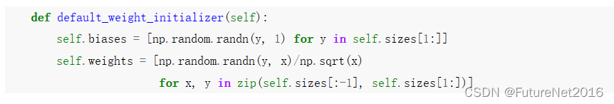
让我们从检查 default_weight_initializer 方法开始。这个方法利用了我们新的、改进过的权重初始化方法。正如我们所见,根据这个方法,输入到神经元的权重被初始化为均值为 0,标准差为 1 再除以神经元输入连接数的平方根的高斯随机变量。在这个方法中,我们也将初始化偏置,使用均值为 0,标准差为 1 的高斯随机变量。以下是代码:
    def default_weight_initializer(self):
        self.biases = [np.random.randn(y, 1) for y in self.sizes[1:]]
        self.weights = [np.random.randn(y, x)/np.sqrt(x)
                        for x, y in zip(self.sizes[:-1], self.sizes[1:])]
为了理解这段代码,回忆一下 np 是用于执行线性代数的 Numpy 库可能会有所帮助。我们将在程序开始时导入 Numpy。此外,请注意,我们不会为第一层神经元初始化任何偏置。我们避免这样做是因为第一层是一个输入层,因此任何偏差都不会被使用。我们在 network.py 中也是这样做的。
作为 default_weight_initializer 的补充,我们还将包括一个 large_weight_initializer 方法。该方法使用了前面的旧方法初始化权重和偏差,其中权重和偏差都被初始化为均值为 0,标准差为 1 的高斯随机变量。当然,代码与 default_weight_initializer 仅有微小的不同:
    def large_weight_initializer(self):
        self.biases = [np.random.randn(y, 1) for y in self.sizes[1:]]
        self.weights = [np.random.randn(y, x)
                        for x, y in zip(self.sizes[:-1], self.sizes[1:])]
我主要包含了 large_weight_initializer 方法,方便在本章中与前面的结果进行比较。
Network 的 init 方法中的第二个新特性是我们现在初始化了一个 cost 属性。为了理解它是如何工作的,让我们来看一下我们用来表示交叉熵损失的类
class CrossEntropyCost(object):

    @staticmethod
    def fn(a, y):
        return np.sum(np.nan_to_num(-y*np.log(a)-(1-y)*np.log(1-a)))

    @staticmethod
    def delta(z, a, y):
        return (a-y)
让我们来分解一下。首先要注意的是,尽管从数学上讲,交叉熵是一个函数,但我们将其实现为一个 Python 类,而不是一个 Python 函数。为什么我会做出这样的选择呢?原因在于成本在我们的网络中扮演了两种不同的角色。显而易见的角色是它是衡量输出激活 a 与期望输出 y 匹配程度的指标。这个角色由 CrossEntropyCost.fn 方法所捕获。(顺便提一句,CrossEntropyCost.fn 内部的 np.nan_to_num 调用确保了 Numpy 正确处理非常接近零的数的对数。)但成本函数进入我们的网络的第二种方式也是重要的。回想一下第二章中提到的,当运行反向传播算法时,我们需要计算网络的输出误差 δ L \delta^L δL。输出误差的形式取决于成本函数的选择:不同的成本函数,输出误差的形式也不同。对于交叉熵,输出误差如我们在方程(66)中看到的那样。
δ L = a L − y . (99) \delta^L = a^L-y.\tag{99} δL=aL−y.(99)
因此,我们定义了第二个方法 CrossEntropyCost.delta,其目的是告诉我们的网络如何计算输出误差。然后,我们将这两个方法捆绑到一个单独的类中,该类包含我们的网络需要了解的有关成本函数的所有信息。
类似地,network2.py 还包含一个用于表示二次成本函数的类。这是为了与第一章的结果进行比较,因为在未来我们将主要使用交叉熵。以下是代码。QuadraticCost.fn 方法是对实际输出 a 和期望输出 y 相关的二次成本的直接计算。QuadraticCost.delta 返回的值基于我们在第前面推导出的二次成本的输出误差的表达式(30)。
class QuadraticCost(object):

    @staticmethod
    def fn(a, y):
        return 0.5*np.linalg.norm(a-y)**2

    @staticmethod
    def delta(z, a, y):
        return (a-y) * sigmoid_prime(z)
现在我们已经了解了 network2.py 和 network.py 之间的主要区别。这都是相当简单的内容。还有一些较小的变化,我将在下面讨论,包括 L2 正则化的实现。在继续讨论之前,让我们看一下 network2.py 的完整代码。您不需要详细阅读所有代码,但了解其大致结构是值得的,特别是阅读文档字符串,这样您就可以理解程序的每个部分正在做什么。当然,您也可以根据需要深入探讨!如果您迷失了方向,可以继续阅读下面的散文,稍后再返回代码。无论如何,以下是代码:
"""network2.py
~~~~~~~~~~~~~~

An improved version of network.py, implementing the stochastic
gradient descent learning algorithm for a feedforward neural network.
Improvements include the addition of the cross-entropy cost function,
regularization, and better initialization of network weights.  Note
that I have focused on making the code simple, easily readable, and
easily modifiable.  It is not optimized, and omits many desirable
features.

"""

#### Libraries
# Standard library
import json
import random
import sys

# Third-party libraries
import numpy as np


#### Define the quadratic and cross-entropy cost functions

class QuadraticCost(object):

    @staticmethod
    def fn(a, y):
        """Return the cost associated with an output ``a`` and desired output
        ``y``.

        """
        return 0.5*np.linalg.norm(a-y)**2

    @staticmethod
    def delta(z, a, y):
        """Return the error delta from the output layer."""
        return (a-y) * sigmoid_prime(z)


class CrossEntropyCost(object):

    @staticmethod
    def fn(a, y):
        """Return the cost associated with an output ``a`` and desired output
        ``y``.  Note that np.nan_to_num is used to ensure numerical
        stability.  In particular, if both ``a`` and ``y`` have a 1.0
        in the same slot, then the expression (1-y)*np.log(1-a)
        returns nan.  The np.nan_to_num ensures that that is converted
        to the correct value (0.0).

        """
        return np.sum(np.nan_to_num(-y*np.log(a)-(1-y)*np.log(1-a)))

    @staticmethod
    def delta(z, a, y):
        """Return the error delta from the output layer.  Note that the
        parameter ``z`` is not used by the method.  It is included in
        the method's parameters in order to make the interface
        consistent with the delta method for other cost classes.

        """
        return (a-y)


#### Main Network class
class Network(object):

    def __init__(self, sizes, cost=CrossEntropyCost):
        """The list ``sizes`` contains the number of neurons in the respective
        layers of the network.  For example, if the list was [2, 3, 1]
        then it would be a three-layer network, with the first layer
        containing 2 neurons, the second layer 3 neurons, and the
        third layer 1 neuron.  The biases and weights for the network
        are initialized randomly, using
        ``self.default_weight_initializer`` (see docstring for that
        method).

        """
        self.num_layers = len(sizes)
        self.sizes = sizes
        self.default_weight_initializer()
        self.cost=cost

    def default_weight_initializer(self):
        """Initialize each weight using a Gaussian distribution with mean 0
        and standard deviation 1 over the square root of the number of
        weights connecting to the same neuron.  Initialize the biases
        using a Gaussian distribution with mean 0 and standard
        deviation 1.

        Note that the first layer is assumed to be an input layer, and
        by convention we won't set any biases for those neurons, since
        biases are only ever used in computing the outputs from later
        layers.

        """
        self.biases = [np.random.randn(y, 1) for y in self.sizes[1:]]
        self.weights = [np.random.randn(y, x)/np.sqrt(x)
                        for x, y in zip(self.sizes[:-1], self.sizes[1:])]

    def large_weight_initializer(self):
        """Initialize the weights using a Gaussian distribution with mean 0
        and standard deviation 1.  Initialize the biases using a
        Gaussian distribution with mean 0 and standard deviation 1.

        Note that the first layer is assumed to be an input layer, and
        by convention we won't set any biases for those neurons, since
        biases are only ever used in computing the outputs from later
        layers.

        This weight and bias initializer uses the same approach as in
        Chapter 1, and is included for purposes of comparison.  It
        will usually be better to use the default weight initializer
        instead.

        """
        self.biases = [np.random.randn(y, 1) for y in self.sizes[1:]]
        self.weights = [np.random.randn(y, x)
                        for x, y in zip(self.sizes[:-1], self.sizes[1:])]

    def feedforward(self, a):
        """Return the output of the network if ``a`` is input."""
        for b, w in zip(self.biases, self.weights):
            a = sigmoid(np.dot(w, a)+b)
        return a

    def SGD(self, training_data, epochs, mini_batch_size, eta,
            lmbda = 0.0,
            evaluation_data=None,
            monitor_evaluation_cost=False,
            monitor_evaluation_accuracy=False,
            monitor_training_cost=False,
            monitor_training_accuracy=False):
        """Train the neural network using mini-batch stochastic gradient
        descent.  The ``training_data`` is a list of tuples ``(x, y)``
        representing the training inputs and the desired outputs.  The
        other non-optional parameters are self-explanatory, as is the
        regularization parameter ``lmbda``.  The method also accepts
        ``evaluation_data``, usually either the validation or test
        data.  We can monitor the cost and accuracy on either the
        evaluation data or the training data, by setting the
        appropriate flags.  The method returns a tuple containing four
        lists: the (per-epoch) costs on the evaluation data, the
        accuracies on the evaluation data, the costs on the training
        data, and the accuracies on the training data.  All values are
        evaluated at the end of each training epoch.  So, for example,
        if we train for 30 epochs, then the first element of the tuple
        will be a 30-element list containing the cost on the
        evaluation data at the end of each epoch. Note that the lists
        are empty if the corresponding flag is not set.

        """
        if evaluation_data: n_data = len(evaluation_data)
        n = len(training_data)
        evaluation_cost, evaluation_accuracy = [], []
        training_cost, training_accuracy = [], []
        for j in xrange(epochs):
            random.shuffle(training_data)
            mini_batches = [
                training_data[k:k+mini_batch_size]
                for k in xrange(0, n, mini_batch_size)]
            for mini_batch in mini_batches:
                self.update_mini_batch(
                    mini_batch, eta, lmbda, len(training_data))
            print "Epoch %s training complete" % j
            if monitor_training_cost:
                cost = self.total_cost(training_data, lmbda)
                training_cost.append(cost)
                print "Cost on training data: {}".format(cost)
            if monitor_training_accuracy:
                accuracy = self.accuracy(training_data, convert=True)
                training_accuracy.append(accuracy)
                print "Accuracy on training data: {} / {}".format(
                    accuracy, n)
            if monitor_evaluation_cost:
                cost = self.total_cost(evaluation_data, lmbda, convert=True)
                evaluation_cost.append(cost)
                print "Cost on evaluation data: {}".format(cost)
            if monitor_evaluation_accuracy:
                accuracy = self.accuracy(evaluation_data)
                evaluation_accuracy.append(accuracy)
                print "Accuracy on evaluation data: {} / {}".format(
                    self.accuracy(evaluation_data), n_data)
            print
        return evaluation_cost, evaluation_accuracy, \
            training_cost, training_accuracy

    def update_mini_batch(self, mini_batch, eta, lmbda, n):
        """Update the network's weights and biases by applying gradient
        descent using backpropagation to a single mini batch.  The
        ``mini_batch`` is a list of tuples ``(x, y)``, ``eta`` is the
        learning rate, ``lmbda`` is the regularization parameter, and
        ``n`` is the total size of the training data set.

        """
        nabla_b = [np.zeros(b.shape) for b in self.biases]
        nabla_w = [np.zeros(w.shape) for w in self.weights]
        for x, y in mini_batch:
            delta_nabla_b, delta_nabla_w = self.backprop(x, y)
            nabla_b = [nb+dnb for nb, dnb in zip(nabla_b, delta_nabla_b)]
            nabla_w = [nw+dnw for nw, dnw in zip(nabla_w, delta_nabla_w)]
        self.weights = [(1-eta*(lmbda/n))*w-(eta/len(mini_batch))*nw
                        for w, nw in zip(self.weights, nabla_w)]
        self.biases = [b-(eta/len(mini_batch))*nb
                       for b, nb in zip(self.biases, nabla_b)]

    def backprop(self, x, y):
        """Return a tuple ``(nabla_b, nabla_w)`` representing the
        gradient for the cost function C_x.  ``nabla_b`` and
        ``nabla_w`` are layer-by-layer lists of numpy arrays, similar
        to ``self.biases`` and ``self.weights``."""
        nabla_b = [np.zeros(b.shape) for b in self.biases]
        nabla_w = [np.zeros(w.shape) for w in self.weights]
        # feedforward
        activation = x
        activations = [x] # list to store all the activations, layer by layer
        zs = [] # list to store all the z vectors, layer by layer
        for b, w in zip(self.biases, self.weights):
            z = np.dot(w, activation)+b
            zs.append(z)
            activation = sigmoid(z)
            activations.append(activation)
        # backward pass
        delta = (self.cost).delta(zs[-1], activations[-1], y)
        nabla_b[-1] = delta
        nabla_w[-1] = np.dot(delta, activations[-2].transpose())
        # Note that the variable l in the loop below is used a little
        # differently to the notation in Chapter 2 of the book.  Here,
        # l = 1 means the last layer of neurons, l = 2 is the
        # second-last layer, and so on.  It's a renumbering of the
        # scheme in the book, used here to take advantage of the fact
        # that Python can use negative indices in lists.
        for l in xrange(2, self.num_layers):
            z = zs[-l]
            sp = sigmoid_prime(z)
            delta = np.dot(self.weights[-l+1].transpose(), delta) * sp
            nabla_b[-l] = delta
            nabla_w[-l] = np.dot(delta, activations[-l-1].transpose())
        return (nabla_b, nabla_w)

    def accuracy(self, data, convert=False):
        """Return the number of inputs in ``data`` for which the neural
        network outputs the correct result. The neural network's
        output is assumed to be the index of whichever neuron in the
        final layer has the highest activation.

        The flag ``convert`` should be set to False if the data set is
        validation or test data (the usual case), and to True if the
        data set is the training data. The need for this flag arises
        due to differences in the way the results ``y`` are
        represented in the different data sets.  In particular, it
        flags whether we need to convert between the different
        representations.  It may seem strange to use different
        representations for the different data sets.  Why not use the
        same representation for all three data sets?  It's done for
        efficiency reasons -- the program usually evaluates the cost
        on the training data and the accuracy on other data sets.
        These are different types of computations, and using different
        representations speeds things up.  More details on the
        representations can be found in
        mnist_loader.load_data_wrapper.

        """
        if convert:
            results = [(np.argmax(self.feedforward(x)), np.argmax(y))
                       for (x, y) in data]
        else:
            results = [(np.argmax(self.feedforward(x)), y)
                        for (x, y) in data]
        return sum(int(x == y) for (x, y) in results)

    def total_cost(self, data, lmbda, convert=False):
        """Return the total cost for the data set ``data``.  The flag
        ``convert`` should be set to False if the data set is the
        training data (the usual case), and to True if the data set is
        the validation or test data.  See comments on the similar (but
        reversed) convention for the ``accuracy`` method, above.
        """
        cost = 0.0
        for x, y in data:
            a = self.feedforward(x)
            if convert: y = vectorized_result(y)
            cost += self.cost.fn(a, y)/len(data)
        cost += 0.5*(lmbda/len(data))*sum(
            np.linalg.norm(w)**2 for w in self.weights)
        return cost

    def save(self, filename):
        """Save the neural network to the file ``filename``."""
        data = {"sizes": self.sizes,
                "weights": [w.tolist() for w in self.weights],
                "biases": [b.tolist() for b in self.biases],
                "cost": str(self.cost.__name__)}
        f = open(filename, "w")
        json.dump(data, f)
        f.close()

#### Loading a Network
def load(filename):
    """Load a neural network from the file ``filename``.  Returns an
    instance of Network.

    """
    f = open(filename, "r")
    data = json.load(f)
    f.close()
    cost = getattr(sys.modules[__name__], data["cost"])
    net = Network(data["sizes"], cost=cost)
    net.weights = [np.array(w) for w in data["weights"]]
    net.biases = [np.array(b) for b in data["biases"]]
    return net

#### Miscellaneous functions
def vectorized_result(j):
    """Return a 10-dimensional unit vector with a 1.0 in the j'th position
    and zeroes elsewhere.  This is used to convert a digit (0...9)
    into a corresponding desired output from the neural network.

    """
    e = np.zeros((10, 1))
    e[j] = 1.0
    return e

def sigmoid(z):
    """The sigmoid function."""
    return 1.0/(1.0+np.exp(-z))

def sigmoid_prime(z):
    """Derivative of the sigmoid function."""
    return sigmoid(z)*(1-sigmoid(z))
代码中的一个更有趣的变化是包含 L2 正则化。尽管这是一个重要的概念性变化,但在代码中实现起来非常微不足道,很容易被忽略。在很大程度上,它只涉及将参数 lambda 传递给各种方法,特别是 Network.SGD 方法。真正的工作是在程序的倒数第四行,也就是 Network.update_mini_batch 方法中完成的。那里我们修改了梯度下降更新规则,以包括权重衰减。尽管修改很小,但对结果影响很大!
顺便说一句,在神经网络中实现新技术时,这是很常见的情况。我们已经花费了成千上万字来讨论正则化。从概念上讲,它相当微妙,难以理解。然而,将其添加到我们的程序中却是微不足道的!令人惊讶的是,复杂的技术经常可以通过对代码进行小幅修改来实现。
我们代码中的另一个小但重要的变化是向随机梯度下降方法 Network.SGD 添加了几个可选标志。这些标志使得可以监视成本和准确度,无论是在训练数据还是在一组评估数据上,后者可以传递给 Network.SGD。我们在本章前面经常使用这些标志,但让我举个例子来说明它的工作原理,只是为了提醒您一下:
>>> import mnist_loader
>>> training_data, validation_data, test_data = \
... mnist_loader.load_data_wrapper()
>>> import network2
>>> net = network2.Network([784, 30, 10], cost=network2.CrossEntropyCost)
>>> net.SGD(training_data, 30, 10, 0.5,
... lmbda = 5.0,
... evaluation_data=validation_data,
... monitor_evaluation_accuracy=True,
... monitor_evaluation_cost=True,
... monitor_training_accuracy=True,
... monitor_training_cost=True)
在这里,我们将 evaluation_data 设置为 validation_data。但我们也可以监视 test_data 或任何其他数据集的性能。我们还有四个标志,告诉我们监视 evaluation_data 和 training_data 上的成本和准确度。这些标志默认为 False,但在这里已经打开,以监视我们网络的性能。此外,network2.py 的 Network.SGD 方法返回一个四元组,表示监视结果。我们可以按如下方式使用它:
>>> evaluation_cost, evaluation_accuracy,
... training_cost, training_accuracy = net.SGD(training_data, 30, 10, 0.5,
... lmbda = 5.0,
... evaluation_data=validation_data,
... monitor_evaluation_accuracy=True,
... monitor_evaluation_cost=True,
... monitor_training_accuracy=True,
... monitor_training_cost=True)
因此,例如,evaluation_cost 将是一个包含每个时期结束时评估数据的成本的 30 个元素的列表。这种信息在理解网络行为方面非常有用。例如,它可以用来绘制显示网络随时间学习情况的图表。实际上,这正是我在前面构建所有图表的方法。然而,请注意,如果任何监视标志未设置,则元组中相应的元素将是空列表。
代码的其他新增内容包括 Network.save 方法,用于将 Network 对象保存到磁盘,并提供加载它们的函数。请注意,保存和加载是使用 JSON 完成的,而不是 Python 的 pickle 或 cPickle 模块,后者是我们在 Python 中通常保存和加载对象到磁盘的方法。使用 JSON 需要比 pickle 或 cPickle 多出更多的代码。为了理解为什么我使用了 JSON,请想象一下,将来我们决定更改我们的 Network 类以允许除 S 型神经元以外的其他神经元。要实现这个变化,我们最有可能更改 Network.init 方法中定义的属性。如果我们只是简单地使用 pickle 对对象进行了序列化,那么会导致我们的加载函数失败。使用 JSON 显式地进行序列化可以轻松确保旧的 Networks 仍然可以加载。
在 network2.py 的代码中还有许多其他较小的变化,但它们都是对 network.py 的简单变化。最终效果是将我们的 74 行程序扩展到了一个更有能力的 152 行。