目标
在本实验中,你将:检查执行情况并利用成本函数进行逻辑回归。
import numpy as np
%matplotlib widget
import matplotlib.pyplot as plt
from lab_utils_common import plot_data, sigmoid, dlc
plt.style.use('./deeplearning.mplstyle')
数据集
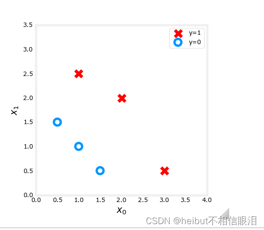
让我们从决策边界实验室中使用的相同数据集开始。
X_train = np.array([[0.5, 1.5], [1,1], [1.5, 0.5], [3, 0.5], [2, 2], [1, 2.5]])  #(m,n)
y_train = np.array([0, 0, 0, 1, 1, 1])                                           #(m,)
我们将使用一个辅助函数来绘制这些数据。标签y = 1的数据点显示为红色标记为y = 0的数据点用蓝色圆圈表示。
成本函数
在之前的实验中,你开发了逻辑损失函数。回想一下,loss被定义为应用于一个示例。在这里,您将损失组合起来形成成本,其中包括所有示例。
回想一下,对于逻辑回归,成本函数是这样的形式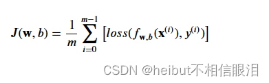

代码描述
compute_cost_logistic循环的算法遍历所有示例,计算每个示例求和的损失。注意变量X和y不是标量值,而是形状分别为(m, n)和(m,)的矩阵,其中n是特征的数量,m是训练样例的数量。
def compute_cost_logistic(X, y, w, b):
    """
    Computes cost

    Args:
      X (ndarray (m,n)): Data, m examples with n features
      y (ndarray (m,)) : target values
      w (ndarray (n,)) : model parameters
      b (scalar)       : model parameter

    Returns:
      cost (scalar): cost
    """

    m = X.shape[0]
    cost = 0.0
    for i in range(m):
        z_i = np.dot(X[i],w) + b
        f_wb_i = sigmoid(z_i)
        cost +=  -y[i]*np.log(f_wb_i) - (1-y[i])*np.log(1-f_wb_i)

    cost = cost / m
    return cost
使用下面的单元格检查成本函数的实现。
w_tmp = np.array([1,1])
b_tmp = -3
print(compute_cost_logistic(X_train, y_train, w_tmp, b_tmp))

例子
现在,让我们看看对于不同的w值,代价函数的输出是什么。
在之前的实验中,您绘制了b = -3, w0 = 1, w1 = 1的决策边界。也就是说,w= np.array([- 3,1,1])。
假设你想知道b = -4, w0 = 1, w1 = 1,或者w = np.Array([- 4,1,1])提供了一个更好的模型。
让我们首先绘制这两个不同b值的决策边界,看看哪一个更适合数据。
- 对于b=-3, w0 =1, w1=1,我们画出-3+xo +x=0(用蓝色表示)
- 对于b=-4, w0=1,w1=1,我们画出-4+xo+x=0(用洋红色表示)
import matplotlib.pyplot as plt

# Choose values between 0 and 6
x0 = np.arange(0,6)

# Plot the two decision boundaries
x1 = 3 - x0
x1_other = 4 - x0

fig,ax = plt.subplots(1, 1, figsize=(4,4))
# Plot the decision boundary
ax.plot(x0,x1, c=dlc["dlblue"], label="$b$=-3")
ax.plot(x0,x1_other, c=dlc["dlmagenta"], label="$b$=-4")
ax.axis([0, 4, 0, 4])

# Plot the original data
plot_data(X_train,y_train,ax)
ax.axis([0, 4, 0, 4])
ax.set_ylabel('$x_1$', fontsize=12)
ax.set_xlabel('$x_0$', fontsize=12)
plt.legend(loc="upper right")
plt.title("Decision Boundary")
plt.show()

你可以从这张图中看到。对于训练数据,Array([- 4,1,1])是一个较差的模型。让我们看看成本函数的实现是否反映了这一点
w_array1 = np.array([1,1])
b_1 = -3
w_array2 = np.array([1,1])
b_2 = -4

print("Cost for b = -3 : ", compute_cost_logistic(X_train, y_train, w_array1, b_1))
print("Cost for b = -4 : ", compute_cost_logistic(X_train, y_train, w_array2, b_2))
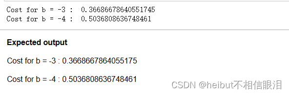
您可以看到成本函数的行为与预期一致,并且成本w = np.array([- 4,1,1])确实比w=np.array[-3,1,1]的代价高
恭喜
在本实验中,您检查并使用了逻辑回归的成本函数。