高维数据的中介效应【中介分析】《R包：HIMA》

2024-02-22 12:42:02
开发
46

允许基于高级中介筛选和惩罚回归技术来估计和测试高维中介效应

Hima包浏览

高维中介示意图

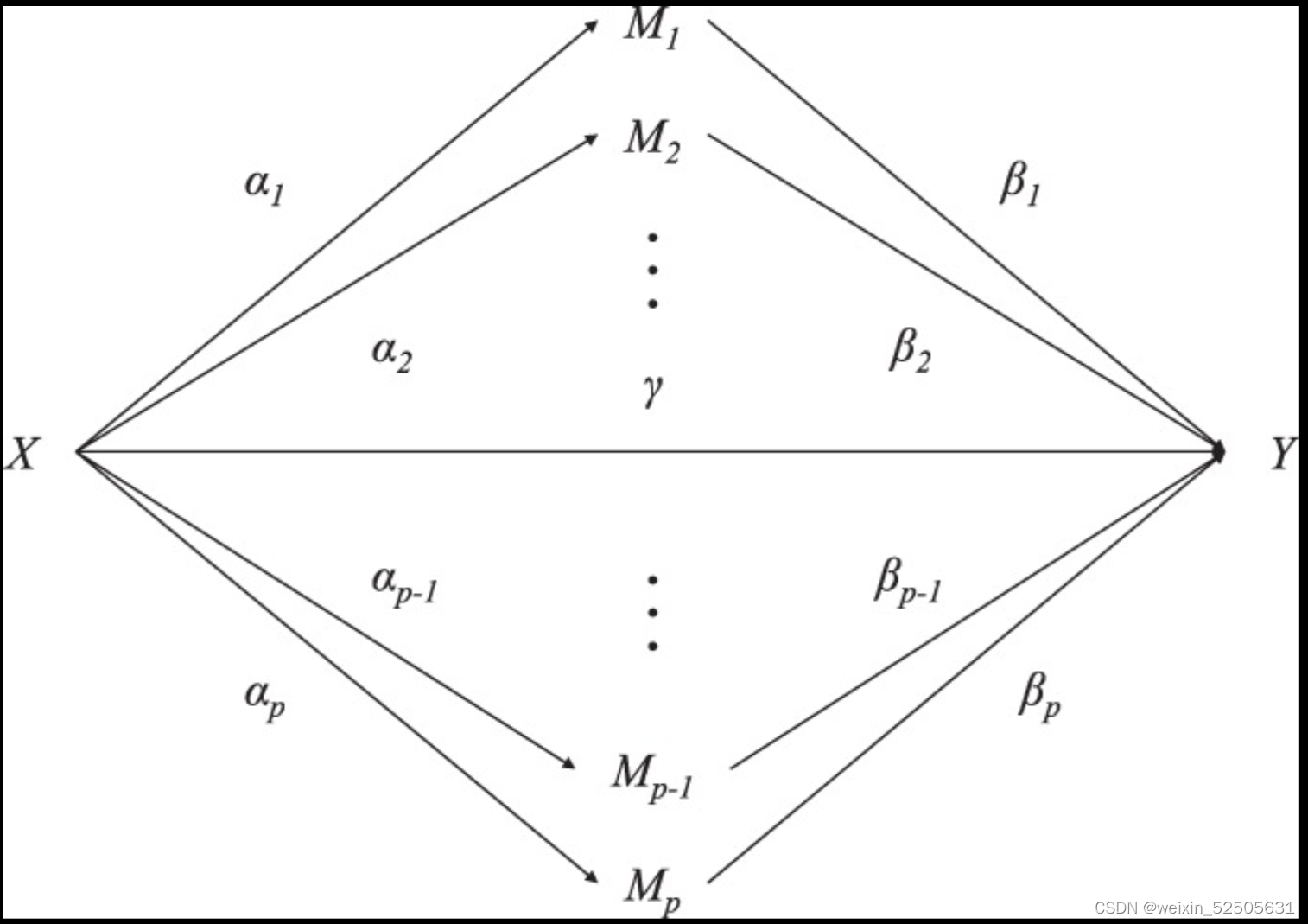
图1. 在暴露和结果之间有高维中介的情况

本包的作用

在确定独立筛选和极小极大凹惩罚技术的基础上，采用联合显著性检验方法对调解效果进行检验。使用蒙特卡罗模拟研究来展示其实际性能，鉴定具有显著中介作用的因子。

分析前准备

# install.packages("HIMA")
# ??hima
library(HIMA)
data(himaDat)

# 熟悉数据
head(himaDat$Example1$PhenoData)
#   Treatment   Outcome Sex Age
# 1         1 2.7653005   0  54
# 2         1 0.5754423   1  38
# 3         1 1.7632589   0  29
# 4         1 9.9327242   0  34
# 5         1 1.8183044   0  29
# 6         1 0.1024832   0  55

dim(himaDat$Example1$PhenoData)
# [1] 300   4
head(himaDat$Example1$Mediator)

glimpse(himaDat$Example1$Mediator)
# num [1:300, 1:300] -2.272 -0.1 0.414 2.275 -0.262 ...
# - attr(*, "dimnames")=List of 2
# ..$ : chr [1:300] "S1" "S2" "S3" "S4" ...
# ..$ : chr [1:300] "M1" "M2" "M3" "M4" ...
dim(himaDat$Example1$Mediator)

dblassoHIMA()

这是使用纠偏LASSO与纠偏LASSO的高维中介分析的函数

纠偏 LASSO (debiased LASSO)

head(himaDat$Example2$PhenoData)

dblassohima.logistic.fit <- dblassoHIMA(X = himaDat$Example2$PhenoData$Treatment,
                                        Y = himaDat$Example2$PhenoData$Disease,
                                        M = himaDat$Example2$Mediator,
                                        Z = himaDat$Example2$PhenoData[, c("Sex", "Age")],
                                        Y.family = 'binomial',
                                        scale = FALSE,
                                        verbose = TRUE)
dblassohima.logistic.fit
# 输出结果
#       alpha        beta    gamma   alpha*beta   % total effect  p.joint
# M1  0.6096868  0.07404941 2.096248 0.04514695       2.153703 1.332402e-03
# M2  0.9677835  0.07339861 2.096248 0.07103396       3.388624 4.330462e-08
# M3 -0.6657028 -0.04116939 2.096248 0.02740657       1.307411 1.244578e-03

Hima()

Hima用于估计和检验高维中介效应。

# hima
# Y：连续性变量------
hima.fit <- hima(X = himaDat$Example1$PhenoData$Treatment, 
                 Y = himaDat$Example1$PhenoData$Outcome, 
                 M = himaDat$Example1$Mediator,
                 COV.XM = himaDat$Example1$PhenoData[, c("Sex", "Age")],
                 Y.family = 'gaussian',
                 scale = FALSE,
                 verbose = TRUE) 
hima.fit
# alpha       beta   gamma alpha*beta % total effect Bonferroni.p       BH.FDR
# M1  0.5771873  0.8917198 2.94202  0.5146893       17.49442 4.844611e-03 1.614870e-03
# M2  0.9137393  0.8461100 2.94202  0.7731240       26.27868 3.279920e-08 3.279920e-08
# M3 -0.7331281 -0.7424343 2.94202  0.5442994       18.50087 1.863286e-04 9.316431e-05

# Y：二分类变量-----
hima.logistic.fit <- hima(X = himaDat$Example2$PhenoData$Treatment,
                          Y = himaDat$Example2$PhenoData$Disease,
                          M = himaDat$Example2$Mediator,
                          COV.XM = himaDat$Example2$PhenoData[, c("Sex", "Age")],
                          Y.family = 'binomial',
                          scale = FALSE,
                          verbose = TRUE)
hima.logistic.fit

# alpha       beta    gamma alpha*beta % total effect Bonferroni.p       BH.FDR
# M1    0.6096868  1.0393063 2.096248  0.6336514      30.227885 5.914712e-03 1.971571e-03
# M2    0.9677835  1.0148114 2.096248  0.9821177      46.851219 3.703063e-07 3.703063e-07
# M3   -0.6657028 -0.4412061 2.096248  0.2937121      14.011326 3.040410e-03 1.013470e-03
# M266 -0.4870164 -0.2619480 2.096248  0.1275729       6.085776 5.480125e-02 1.370031e-02

hima2()

是hima的升级版，用于评估和检验高维中介效应，支持公式输入

#hima2 
# Y: 连续性变量--------
e1 <- hima2(Outcome ~ Treatment + Sex + Age, 
            data.pheno = himaDat$Example1$PhenoData, 
            data.M = himaDat$Example1$Mediator,
            outcome.family = "gaussian",
            mediator.family = "gaussian",
            penalty = "DBlasso",
            scale = FALSE) # Disabled only for example data
e1
attributes(e1)$variable.labels

# Y: 二分类变量--------
e2 <- hima2(Disease ~ Treatment + Sex + Age, 
            data.pheno = himaDat$Example2$PhenoData, 
            data.M = himaDat$Example2$Mediator,
            outcome.family = "binomial",
            mediator.family = "gaussian",
            penalty = "DBlasso",
            scale = FALSE) # Disabled only for example data
e2
attributes(e2)$variable.labels

# Y: 生存型变量--------

e3 <- hima2(Surv(Status, Time) ~ Treatment + Sex + Age, 
            data.pheno = himaDat$Example3$PhenoData, 
            data.M = himaDat$Example3$Mediator,
            outcome.family = "survival",
            mediator.family = "gaussian",
            penalty = "DBlasso",
            scale = FALSE) # Disabled only for example data
e3
attributes(e3)$variable.labels

# M: 中介变量属于Compositional data--------
# Compositional data是指数据记录了一个整体（或者样本）中各个组成部分的相对比例信息。这些数据通常用来描述某些总和为常数（例如100%或者1）的组分。这种类型的数据在不同的领域中都有出现，例如地质学、环境学、生态学和生物信息学中的微生物组数据分析。
# 微生物组数据，也就是关于一个环境（比如说人体肠道）中微生物群落的组成信息，是compositional data的一个典型例子。compositional data的一个关键特性是它们的组分是相对测量的而不是绝对测量的。这就意味着，当一个组分的比例增加时，至少有一个其他组分的比例必定减少，因为它们的总和是一个固定的常数。这种数据的这个特性导致它不能直接像其他类型的数据那样进行分析，因为传统的统计方法往往假定数据是独立的和不受限的。因此，为了分析compositional data，需要使用专门的数学方法和统计模型，例如对数比率分析（log-ratio analysis），本方法使用isometric logratio (ilr)-based transformation (等距对数比)进行分析。

e4 <- hima2(Outcome ~ Treatment + Sex + Age, 
            data.pheno = himaDat$Example4$PhenoData, 
            data.M = himaDat$Example4$Mediator,
            outcome.family = "gaussian",
            mediator.family = "compositional",
            penalty = "DBlasso",
            scale = FALSE) # Disabled only for example data
e4
attributes(e4)$variable.labels

# Y: 分位数水平变量

# Note that the function will prompt input for quantile level.
e5 <- hima2(Outcome ~ Treatment + Sex + Age, 
            data.pheno = himaDat$Example5$PhenoData, 
            data.M = himaDat$Example5$Mediator,
            outcome.family = "quantile",
            mediator.family = "gaussian",
            penalty = "MCP", # Quantile HIMA does not support DBlasso
            scale = FALSE, # Disabled only for example data
            tau = c(0.3, 0.5, 0.7)) # Specify multiple quantile level
e5
attributes(e5)$variable.labels

qHIMA()

这是第2种方法：用于估计和检验高维分位数的中介效应。[注：第1种方法：hima2()]

# qHIMA
head(himaDat$Example5$PhenoData)
# 【结果输出】
#   Treatment  Outcome Sex Age
# 1         1 16.18104   1  23
# 2         1 18.60296   0  20
# 3         1 28.80309   1  42
# 4         1 26.38711   0  34
# 5         1 25.29259   0  44
# 6         1 42.41721   1  61

qHIMA.fit <- qHIMA(X = himaDat$Example5$PhenoData$Treatment,
                   M = himaDat$Example5$Mediator, 
                   Y = himaDat$Example5$PhenoData$Outcome, 
                   Z = himaDat$Example5$PhenoData[, c("Sex", "Age")], 
                   Bonfcut = 0.05,
                   tau = c(0.3, 0.5, 0.7),
                   scale = FALSE, 
                   verbose = TRUE)
qHIMA.fit
# 【结果输出】
#   ID      alpha  alpha_se       beta   beta_se Bonferroni.p tau
# 1 M1  0.7940567 0.1428952  0.7947046 0.1294236 2.745815e-08 0.3
# 2 M2  0.8084565 0.1431067  0.8270942 0.1378767 1.610791e-08 0.3
# 3 M3 -1.1375897 0.1438286 -0.8098622 0.1349740 1.971560e-09 0.3
# 4 M1  0.7940567 0.1428952  0.8696986 0.1481069 2.745815e-08 0.5
# 5 M2  0.8084565 0.1431067  0.7351953 0.1309730 1.984654e-08 0.5
# 6 M1  0.7940567 0.1428952  0.9196337 0.2423962 1.482827e-04 0.7
# 7 M3 -1.1375897 0.1438286 -0.9171627 0.2544897 3.134432e-04 0.7

survHIMA()

这是第2种方法：用于评估和检验生存数据的高维中介效应。[注：第1种方法：hima2()]

head(himaDat$Example3$PhenoData)
# 【结果输出】
#    Treatment Status        Time Sex Age
# 1         0   TRUE 0.034300778   1  31
# 2         0   TRUE 0.497066963   1  51
# 3         1   TRUE 0.046356567   1  39
# 4         1   TRUE 0.024704873   1  22
# 5         0   TRUE 0.126670360   1  26
# 6         1   TRUE 0.007228506   0  60

survHIMA.fit <- survHIMA(X = himaDat$Example3$PhenoData$Treatment,
                         Z = himaDat$Example3$PhenoData[, c("Sex", "Age")], 
                         M = himaDat$Example3$Mediator, 
                         OT = himaDat$Example3$PhenoData$Time, 
                         status = himaDat$Example3$PhenoData$Status, 
                         FDRcut = 0.05,
                         scale = FALSE, 
                         verbose = TRUE)
survHIMA.fit
# 【结果输出】
# ID      alpha  alpha_se       beta    beta_se      p.joint
# 1 M1  1.0384367 0.1365431  0.7940717 0.08687706 2.842171e-14
# 2 M2  0.6414393 0.1507081  0.7969670 0.07691991 2.079579e-05
# 3 M3 -0.9087889 0.1463872 -0.9952480 0.08084286 5.362315e-10

参考文献

Zhang H, Zheng Y, Zhang Z, Gao T, Joyce B, Yoon G, Zhang W, Schwartz J, Just A, Colicino E, Vokonas P, Zhao L, Lv J, Baccarelli A, Hou L, Liu L. Estimating and Testing High dimensional Mediation Effects in Epigenetic Studies. Bioinformatics. (2016) . PMID: 2735717

摘要：

目的：高维 DNA 甲基化标记可能介导环境暴露与健康结果之间的结合。然而，缺乏分析方法来确定高维调解分析的重要中介。

结果: 在确定独立筛选和极小极大凹惩罚技术的基础上，采用联合显著性检验方法对调解效果进行检验。我们使用蒙特卡罗模拟研究来展示其实际性能，并应用这种方法来调查在规范老化研究中，DNA 甲基化标记介导从吸烟到肺功能减少的因果途径的程度。我们鉴定了2个具有显著中介作用的 CpG。

可用性和实现: R 软件包、源代码和模拟研究 https://github.com/yinanzheng/hima

HIMA: High-Dimensional Mediation Analysis (r-project.org)https://cran.r-project.org/web/packages/HIMA/HIMA.pdf

原文地址:https://blog.csdn.net/weixin_52505631/article/details/136185508 本文来自互联网用户投稿，该文观点仅代表作者本人，不代表本站立场。本站仅提供信息存储空间服务，不拥有所有权，不承担相关法律责任。如若转载，请注明出处：https://www.suanlizi.com/kf/1760525327630733312.html 如若内容造成侵权/违法违规/事实不符，请联系《酸梨子》网邮箱：1419361763@qq.com进行投诉反馈，一经查实，立即删除！

阅读全部