20240219画图程序

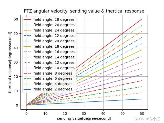
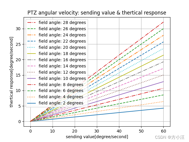
1. PTZ在惯性态时，不同视场角下的【发送】角速度和【理论响应】角速度

1.1 优化前

import numpy as np
import matplotlib.pyplot as plt

# PTZ在惯性态时，不同视场角下的【发送】角速度和【理论响应】角速度
ATROffset_x = np.linspace(0, 60, 120)
y2 = ATROffset_x * 2 / 28
y4 = ATROffset_x * 4 / 28
y6 = ATROffset_x * 6 / 28
y8 = ATROffset_x * 8 / 28
y10 = ATROffset_x * 10 / 28
y12 = ATROffset_x * 12 / 28
y14 = ATROffset_x * 14 / 28
y16 = ATROffset_x * 16 / 28
y18 = ATROffset_x * 18 / 28
y20 = ATROffset_x * 20 / 28
y22 = ATROffset_x * 22 / 28
y24 = ATROffset_x * 24 / 28
y26 = ATROffset_x * 26 / 28
y28 = ATROffset_x * 28 / 28

plt.plot(ATROffset_x, y2, label='field angle: 2 degrees')
plt.plot(ATROffset_x, y4, linestyle='dotted',label='field angle: 4 degrees')
plt.plot(ATROffset_x, y6, linestyle='--',label='field angle: 6 degrees')
plt.plot(ATROffset_x, y8, linestyle='-.', label='field angle: 8 degrees')

plt.plot(ATROffset_x, y10, label='field angle: 10 degrees')
plt.plot(ATROffset_x, y12, linestyle='dotted', label='field angle: 12 degrees')
plt.plot(ATROffset_x, y14, linestyle='--',label='field angle: 14 degrees')
plt.plot(ATROffset_x, y16, linestyle='-.', label='field angle: 16 degrees')

plt.plot(ATROffset_x, y18, label='field angle: 18 degrees')
plt.plot(ATROffset_x, y20, linestyle='dotted', label='field angle: 20 degrees')
plt.plot(ATROffset_x, y22, linestyle='--',label='field angle: 22 degrees')
plt.plot(ATROffset_x, y24, linestyle='-.', label='field angle: 24 degrees')

plt.plot(ATROffset_x, y26, linestyle='dotted', label='field angle: 26 degrees')
plt.plot(ATROffset_x, y28, label='field angle: 28 degrees')

plt.xlabel('sending value[degree/second]')
plt.ylabel('thertical response[degree/second]')
plt.title('PTZ angular velocity: sending value & thertical response')
handles, labels = plt.gca().get_legend_handles_labels()
# plt.legend(handles[::-1], labels[::-1],loc='right')
plt.legend(handles[::-1], labels[::-1])
plt.grid()
plt.show()

1.2 优化后

import numpy as np
import matplotlib.pyplot as plt

ATROffset_x = np.linspace(0, 60, 120)
linestyles = ['-', 'dotted', '--', '-.', 
              '-', 'dotted', '--', '-.', 
              '-', 'dotted', '--', '-.', 
              '-', 'dotted']
labels = [f'field angle: {
     i} degrees' for i in range(2, 30, 2)]

for i, linestyle in enumerate(linestyles):
    y = ATROffset_x * (i + 2) / 28
    plt.plot(ATROffset_x, y, linestyle=linestyle, label=labels[i])

plt.xlabel('sending value[degree/second]')
plt.ylabel('thertical response[degree/second]')
plt.title('PTZ angular velocity: sending value & thertical response')
handles, labels = plt.gca().get_legend_handles_labels()
plt.legend(handles[::-1], labels[::-1])
plt.grid()
plt.show()

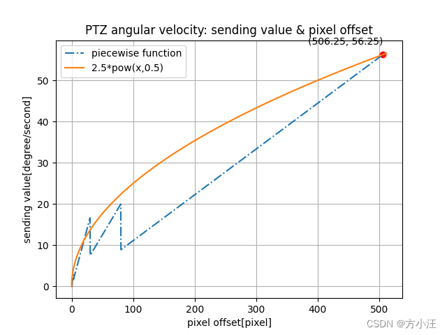
2. 像素偏移与发送角速度

import numpy as np
import matplotlib.pyplot as plt

# 分段函数
def piecewise_function(x):
    if x >80: return x/9
    elif x>30: return x/4
    elif x>10: return x/1.8
    elif x>3: return x/1.8
    elif x>1: return x
    else: return 0

# 生成x值
x = np.linspace(0, 512, 2000)
# 计算y值
y1 = [piecewise_function(xi) for xi in x]
y2 = 2.5*(x**(0.5))
# y3 = 2.5*(x**(0.8))

points = [(506.25, piecewise_function(506.25))]
for point in points:
    plt.plot(point[0], point[1], 'ro')
    plt.annotate(f'({
     point[0]}, {
     point[1]:.2f})', (point[0], point[1]), textcoords="offset points", xytext=(0,10), ha='center')

# 绘制图形
plt.plot(x, y1, label='piecewise function', linestyle='-.')
plt.plot(x, y2, label='2.5*pow(x,0.5)')
# plt.plot(x, y3, label='x**0.8')

plt.xlabel('pixel offset[pixel]')
plt.ylabel('sending value[degree/second]')
plt.title('PTZ angular velocity: sending value & pixel offset')
plt.grid()
plt.legend()
plt.show()

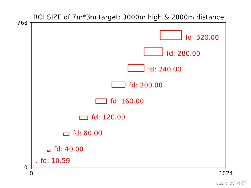
3. 估算不同焦距下的目标大小

3.1 原理

• 【任务】：已知POD与目标之间的高度差3000m和水平距离2000m，需要解算7m*3m目标在POD观察画面中的大小
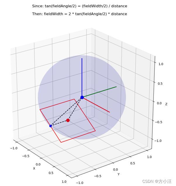
• 【途径】：利用视场角解算视野大小，绘制目标在POD观察画面中的大小
  • 解算视场角大小：
    • fieldAngle_yaw = arctan(5.632/focalDistance)*180/Pi
    • fieldAngle_pitch = arctan(4.224/focalDistance)*180/Pi
  • 解算POD与目标的直线距离distance
  • 解算视野覆盖的实际长和宽
    • fieldWidth = 2*tan(fieldAngle_yaw/2)/disctance
    • fieldWidth = 2*tan(fieldAngle_pitch/2)/disctance
  • 解算目标在视野中的比例后，可得3.2中的图像

import numpy as np
import matplotlib.pyplot as plt
from mpl_toolkits.mplot3d import Axes3D

# 参数方程定义的单位球面
def sphere(u, v):
    theta = u * 2 * np.pi
    phi = v * np.pi
    x = np.sin(phi) * np.cos(theta)
    y = np.sin(phi) * np.sin(theta)
    z = np.cos(phi)
    return x, y, z

def plot_rectangle_tangent_to_point(point):
    # 计算点到原点的单位向量
    point_normalized = point / np.linalg.norm(point)

    # 找到一个与点到原点的向量垂直的向量
    perpendicular_vector_1 = np.cross(point_normalized, [1, 0, 0])
    if np.allclose(perpendicular_vector_1, [0, 0, 0]):
        # 如果点到原点的向量与[1, 0, 0]平行，则选择[0, 1, 0]作为第二个向量
        perpendicular_vector_1 = np.cross(point_normalized, [0, 1, 0])
    perpendicular_vector_1 /= np.linalg.norm(perpendicular_vector_1)

    # 找到与第一个向量垂直的第二个向量
    perpendicular_vector_2 = np.cross(point_normalized, perpendicular_vector_1)
    perpendicular_vector_2 /= np.linalg.norm(perpendicular_vector_2)

    # 生成矩形的四个顶点
    rectangle_half_side = 0.5  # 矩形边长的一半
    rectangle_vertices = np.array([
        point_normalized + rectangle_half_side * perpendicular_vector_1 + rectangle_half_side * perpendicular_vector_2,
        point_normalized - rectangle_half_side * perpendicular_vector_1 + rectangle_half_side * perpendicular_vector_2,
        point_normalized - rectangle_half_side * perpendicular_vector_1 - rectangle_half_side * perpendicular_vector_2,
        point_normalized + rectangle_half_side * perpendicular_vector_1 - rectangle_half_side * perpendicular_vector_2,
        point_normalized + rectangle_half_side * perpendicular_vector_1 + rectangle_half_side * perpendicular_vector_2  # 重复第一个点以闭合图形
    ])

    # 绘制矩形切面
    fig = plt.figure(figsize=(10, 10))
    ax = fig.add_subplot(111, projection='3d')
    ax.plot(rectangle_vertices[:, 0], rectangle_vertices[:, 1], rectangle_vertices[:, 2], color='r')
    ax.scatter(point[0], point[1], point[2], color='b', s=50)  # 绘制点

    # 定义两个点
    point1 = point
    point2 = np.array([0, 0, 0])
    # 绘制两个点
    ax.scatter(point1[0], point1[1], point1[2], color='r', s=100)
    ax.scatter(point2[0], point2[1], point2[2], color='b', s=100)
    # 绘制连线
    ax.plot([point1[0], point2[0]], [point1[1], point2[1]], [point1[2], point2[2]], color='k', linestyle='--')

    # 绘制中点
    fyo = (point_normalized + rectangle_half_side * perpendicular_vector_1 + rectangle_half_side * perpendicular_vector_2 + point_normalized + rectangle_half_side * perpendicular_vector_1 - rectangle_half_side * perpendicular_vector_2)/2
    ax.scatter(fyo[0], fyo[1], fyo[2], color='b', s=50)  # 绘制点
    # 绘制连线
    ax.plot([fyo[0], point2[0]], [fyo[1], point2[1]], [fyo[2], point2[2]], color='k', linestyle='--')
    # 绘制连线-平面内
    ax.plot([fyo[0], point[0]], [fyo[1], point[1]], [fyo[2], point[2]], color='k', linestyle='--')
      
    # 创建参数
    u = np.linspace(0, 2, 100)
    v = np.linspace(0, 2, 100)
    u, v = np.meshgrid(u, v)

    # 计算球面上的点
    x, y, z = sphere(u, v)

    # 绘制单位球面
    ax.plot_surface(x, y, z, color='b', alpha=0.02)
    # 画出xyz轴
    ax.plot([0, 1], [0, 0], [0, 0], color='red', linestyle='-', linewidth=2)
    ax.plot([0, 0], [0, 1], [0, 0], color='green', linestyle='-', linewidth=2)
    ax.plot([0, 0], [0, 0], [0, 1], color='blue', linestyle='-', linewidth=2)
    
    # 设置坐标轴等比例
    ax.set_box_aspect([1,1,1])

    # 设置坐标轴标签
    ax.set_xlabel('X')
    ax.set_ylabel('Y')
    ax.set_zlabel('Z')

    # 设置x轴的刻度
    ax.set_xticks([-1, -0.5, 0, 0.5, 1])
    # 设置y轴的刻度
    ax.set_yticks([-1, -0.5, 0, 0.5, 1])
    # 设置z轴的刻度
    ax.set_zticks([-1, -0.5, 0, 0.5, 1])

    # 设置标题
    plt.title("Since: tan(fieldAngle/2) = (fieldWidth/2) / distance\n\nThen: fieldWidth = 2 * tan(fieldAngle/2) * distance")

    plt.show()

point_on_sphere = np.array([-0.55, 0, -0.83])
plot_rectangle_tangent_to_point(point_on_sphere)

3.2 绘图

• POD与目标之间高度差3000m、水平距离2000m，目标尺寸7m*3m
• 不同焦距下，该目标在POD观察画面中的大小如图所示

import matplotlib.pyplot as plt
import matplotlib.patches as patches
import numpy as np
import math

relative_target_height = 3000
relative_target_horizontal = 2000
relative_distance = math.sqrt(relative_target_height*relative_target_height + relative_target_horizontal*relative_target_horizontal)
print("relative_distance: ", relative_distance)

fig, ax = plt.subplots()# 创建一个新的图形
plt.title("ROI SIZE of 7m*3m target: 3000m high & 2000m distance")# 设置标题

def fd2pic(fd):
    horizontal_draw = np.tan(math.atan(5.632/fd)/2) * relative_distance * 2
    vertical_draw = np.tan(math.atan(4.224/fd)/2) * relative_distance * 2
    # 添加第一个框
    rect = patches.Rectangle((6*7/horizontal_draw*1024, 14*3/vertical_draw*768), 
                             7/horizontal_draw*1024, 3/vertical_draw*768, linewidth=1, edgecolor='r', facecolor='none')
    ax.add_patch(rect)
    # 在第一个框旁边打印文字
    ax.text(7*7/horizontal_draw*1024+20, 14*3/vertical_draw*768, "fd: {:.2f}".format(fd), fontsize=12, color='r')

for i in range(9):
    fd2pic(max(40*i,10.59))

plt.xlim(0, 1024)
plt.ylim(0, 768)
plt.xticks([0, 1024])
plt.yticks([0, 768])
plt.show()