第一题:支持向量机的核函数
实验内容:
- 了解核函数对SVM的影响
- 绘制不同核函数的决策函数图像
- 简述引入核函数的目的
1. 导入模型
import numpy as np
import matplotlib.pyplot as plt
%matplotlib inline
from matplotlib.colors import ListedColormap

import warnings
warnings.filterwarnings('ignore')
# 引入数据集
from sklearn.datasets import make_moons
# 引入数据预处理工具
from sklearn.model_selection import train_test_split
from sklearn.preprocessing import StandardScaler
# 引入支持向量机分类器
from sklearn.svm import SVC
2. 生成数据
X, y = make_moons(n_samples = 100, noise = 0.3, random_state = 0)

plt.figure(figsize = (8, 8))
cm_bright = ListedColormap(['#FF0000', '#0000FF'])
plt.scatter(X[:, 0], X[:, 1], c = y, cmap = cm_bright, edgecolors = 'k')
3. 数据预处理与划分
使用标准化,60%训练集,40%测试集,固定一个随机种子
# YOUR CODE HERE
scaler = StandardScaler()
X = scaler.fit_transform(X)
X_train, X_test, y_train, y_test = train_test_split(X, y, test_size=0.4, random_state=42)
训练集和测试集可视化
cm = plt.cm.RdBu
cm_bright = ListedColormap(['#FF0000', '#0000FF'])
plt.figure(figsize = (8, 8))
plt.title("Input data")
# Plot the training points
plt.scatter(X_train[:, 0], X_train[:, 1], c=y_train, cmap=cm_bright, edgecolors='k')
# and testing points
plt.scatter(X_test[:, 0], X_test[:, 1], c=y_test, cmap=cm_bright, alpha=0.5, edgecolors='k')
4. 样本到分离超平面距离的可视化
我们使用SVM模型里面的decision_function方法,可以获得样本到分离超平面的距离。
下面的函数将图的背景变成数据点,计算每个数据点到分离超平面的距离,映射到不同深浅的颜色上,绘制出了不同颜色的背景。
def plot_model(model, title):

    # 训练模型,计算精度
    # YOUR CODE HERE
    model.fit(X_train, y_train)
    score_train = model.score(X_train, y_train)
    score_test = model.score(X_test, y_test)

    # 将背景网格化
    h = 0.02
    x_min, x_max = X[:, 0].min() - .5, X[:, 0].max() + .5
    y_min, y_max = X[:, 1].min() - .5, X[:, 1].max() + .5
    xx, yy = np.meshgrid(np.arange(x_min, x_max, h),
                         np.arange(y_min, y_max, h))

    # 计算每个点到分离超平面的距离
    # YOUR CODE HERE
    Z = model.decision_function(np.c_[xx.ravel(), yy.ravel()])
    Z = Z.reshape(xx.shape)

    # 设置图的大小
    plt.figure(figsize = (14, 6))

    # 绘制训练集的子图
    plt.subplot(121)

    # 绘制决策边界
    plt.contourf(xx, yy, Z, cmap = cm, alpha=.8)

    # 绘制训练集的样本
    plt.scatter(X_train[:, 0], X_train[:, 1], c=y_train, cmap=cm_bright, edgecolors='k')

    # 设置图的上下左右界
    plt.xlim(xx.min(), xx.max())
    plt.ylim(yy.min(), yy.max())

    # 设置子图标题
    plt.title("training set")

    # 图的右下角写出在当前数据集中的精度
    plt.text(xx.max() - .3, yy.min() + .3, ('acc: %.3f' % score_train).lstrip('0'), size=15, horizontalalignment='right')

    plt.subplot(122)
    plt.contourf(xx, yy, Z, cmap = cm, alpha=.8)

    plt.scatter(X_test[:, 0], X_test[:, 1], c=y_test, cmap=cm_bright, edgecolors='k', alpha=0.6)

    plt.xlim(xx.min(), xx.max())
    plt.ylim(yy.min(), yy.max())

    plt.title("testing set")

    plt.text(xx.max() - .3, yy.min() + .3, ('acc: %.3f' % score_test).lstrip('0'), size=15, horizontalalignment='right')

    plt.suptitle(title)
我们尝试绘制线性核的分类效果图
plot_model(SVC(kernel = "linear", probability = True), 'Linear SVM')
作业1:请你尝试使用其他的核函数,绘制分类效果图
1. 高斯核,又称径向基函数(Radial Basis Function),指定kernel为"rbf"即可
# YOUR CODE HERE
plot_model(SVC(kernel = "rbf", probability = True), 'Linear SVM')
2. sigmoid核,指定kernel为"sigmoid"即可
# YOUR CODE HERE
plot_model(SVC(kernel = "sigmoid", probability = True), 'Linear SVM')
3. 多项式核,指定kernel为"poly"即可
# YOUR CODE HERE
plot_model(SVC(kernel = "poly", probability = True), 'Linear SVM')
作业2:简述为什么要引入核函数?
第二题:支持向量机的软间隔
实验内容:
- 了解分离超平面、间隔超平面与支持向量的绘制
- 调整C的值,绘制分离超平面、间隔超平面和支持向量
- 简述引入软间隔的原因,以及C值对SVM的影响
1. 导入模型
import numpy as np
import matplotlib.pyplot as plt
%matplotlib inline
from sklearn.svm import SVC
2. 制造数据集
np.random.seed(2)
X = np.r_[np.random.randn(20, 2) - [0, 2], np.random.randn(20, 2) + [0, 2]]
Y = [0] * 20 + [1] * 20

def plot_data(X, Y):
    # 新建一个 8 × 8 的图
    plt.figure(figsize = (8, 8))

    # 绘制散点图
    plt.scatter(X[:, 0], X[:, 1], c = Y, cmap = plt.cm.Paired, edgecolors = 'k')

    # 设置横纵坐标标签
    plt.xlabel('x1')
    plt.ylabel('x2')

    # 设定图的范围
    plt.xlim((-4, 4))
    plt.ylim((-4, 4))

plot_data(X, Y)
3. 训练模型
这里我们使用线性核函数,C设定为100
# 创建模型
clf = SVC(kernel = 'linear', C = 100, random_state = 32)
# 训练模型
clf.fit(X, Y)
4. 绘制超平面
在二维平面中,我们将SVM参数写为 w 0 w_0 w0和 w 1 w_1 w1,截距为 b b b。
超平面方程为:
w T x + b = 0 w^{\mathrm{T}} x + b = 0 wTx+b=0
写成分量形式为:
w 0 x 1 + w 1 x 2 + b = 0 w_0 x_1 + w_1 x_2 + b = 0 w0x1+w1x2+b=0
等价于:
x 2 = − w 0 w 1 x 1 − b w 1 x_2 = - \frac{w_0}{w_1} x_1 - \frac{b}{w_1} x2=−w1w0x1−w1b
所以我们可以在上面的图中,绘制这个分离超平面,上图中,纵坐标为 x 2 x_2 x2,横坐标为 x 1 x_1 x1,我们可以通过SVC的coef_属性获取 w w w,通过intercept_获取 b b b。
画图的时候我们可以给定任意两点,如x1等于-5和5的点,计算出这两个点的x2值,然后通过连线的方式,绘制出超平面
def compute_hyperplane(model, x1):
    '''
    计算二维平面上的分离超平面,
    我们通过w0,w1,b以及x1计算出x2,只不过这里的x1是一个ndarray,x2也是一个ndarray

    Parameters
    ----------
    model: sklearn中svm的模型

    x1: numpy.ndarray,如[-5, 5],表示超平面上这些点的横坐标

    Returns
    ----------
    x2: numpy.ndarray, 对应的纵坐标

    '''
    w0 = model.coef_[0][0]
    w1 = model.coef_[0][1]
    b = model.intercept_[0]

    # YOUR CODE HERE
    x2 = (-w0/w1) * x1 - b/w1

    return x2
# 测试样例
x1t = np.array([-5, 5])
x2t = compute_hyperplane(clf, x1t)
print(x2t) # [ 2.05713424 -2.27000147]
# 绘制数据
plot_data(X, Y)
# 在横坐标上选两个点
x1 = np.array([-5, 5])
# 计算超平面上这两个点的对应纵坐标
x2 = compute_hyperplane(clf, x1)
# 绘制这两点连成的直线
plt.plot(x1, x2, '-', color = 'red')
5. 绘制间隔
根据SVM的原理,间隔超平面的方程是:
w T x + b = ± 1 w^{\mathrm{T}}x + b = \pm 1 wTx+b=±1
我们先讨论右侧为1的情况:
w T x + b = 1 w^{\mathrm{T}}x + b = 1 wTx+b=1
写成分量形式:
w 0 x 1 + w 1 x 2 + b = 1 w_0 x_1 + w_1 x_2 + b = 1 w0x1+w1x2+b=1
根据上面第四节的变换,可以得到:
x 2 = 1 w 1 − w 0 w 1 x 1 − b w 1 x2 = \frac{1}{w_1} - \frac{w_0}{w_1} x_1 - \frac{b}{w_1} x2=w11−w1w0x1−w1b
同理,当右侧为-1时,可得:
x 2 = − 1 w 1 − w 0 w 1 x 1 − b w 1 x2 = - \frac{1}{w_1} - \frac{w_0}{w_1} x_1 - \frac{b}{w_1} x2=−w11−w1w0x1−w1b
可以发现,间隔超平面的方程就是在分离超平面上增加或减去 1 w 1 \frac{1}{w_1} w11
def compute_margin(model, x1):
    '''
    计算二维平面上的间隔超平面,
    我们通过w0,w1,b以及x1计算出x2,只不过这里的x1是一个ndarray,x2也是一个ndarray

    Parameters
    ----------
    model: sklearn中svm的模型

    x1: numpy.ndarray,如[-5, 5],表示超平面上这些点的横坐标

    Returns
    ----------
    x2_up: numpy.ndarray, 一条间隔超平面上对应的纵坐标

    x2_down: numpy.ndarray, 另一条间隔超平面上对应的纵坐标

    '''

    # 先调用compute_hyperplane计算超平面的纵坐标
    x2 = compute_hyperplane(model, x1)

    w1 = model.coef_[0][1]

    # YOUR CODE HERE
    # 计算上间隔超平面的纵坐标
    x2_up = x2 + (1/w1)

    # YOUR CODE HERE
    # 计算下间隔超平面的纵坐标
    x2_down = x2 - (1/w1)

    return x2_up, x2_down
# 测试样例
x1t = np.array([-5, 5])
x2_upt, x2_downt = compute_margin(clf, x1t)
print(x2_upt)     # [ 2.43100836 -1.89612735]
print(x2_downt)   # [ 1.68326012 -2.64387559]
# 绘制数据
plot_data(X, Y)

# 在横坐标上选两个点
x1 = np.array([-5, 5])

# 计算超平面上这两个点的对应纵坐标
x2 = compute_hyperplane(clf, x1)

# 计算间隔超平面上这两个点的对应纵坐标
x2_up, x2_down = compute_margin(clf, x1)

# 绘制分离超平面和间隔超平面
plt.plot(x1, x2, '-', color = 'red')
plt.plot(x1, x2_up, 'k--')
plt.plot(x1, x2_down, 'k--')
6. 标出支持向量
模型的support_vectors_属性包含了支持向量
# 绘制数据
plot_data(X, Y)

# 在横坐标上选两个点
x1 = np.array([-5, 5])

# 计算超平面上这两个点的对应纵坐标
x2 = compute_hyperplane(clf, x1)

# 计算间隔超平面上这两个点的对应纵坐标
x2_up, x2_down = compute_margin(clf, x1)

# 绘制分离超平面和间隔超平面
plt.plot(x1, x2, '-', color = 'red')
plt.plot(x1, x2_up, 'k--')
plt.plot(x1, x2_down, 'k--')

# 标出支持向量
plt.scatter(clf.support_vectors_[:, 0], clf.support_vectors_[:, 1], s = 200, facecolors = 'none', edgecolors = 'red')
作业1:请你使用线性核,调整C的值,绘制数据集,SVM分离超平面,间隔超平面以及支持向量
1. C = 10
# YOUR CODE HERE
# 创建模型
clf10 = SVC(kernel = 'linear', C = 10, random_state = 32)
# 训练模型
clf10.fit(X, Y)
# 绘制数据
plot_data(X, Y)

# 在横坐标上选两个点
x10 = np.array([-5, 5])

# 计算超平面上这两个点的对应纵坐标
x20 = compute_hyperplane(clf10, x10)

# 计算间隔超平面上这两个点的对应纵坐标
x20_up, x20_down = compute_margin(clf10, x10)

# 绘制分离超平面和间隔超平面
plt.plot(x10, x20, '-', color = 'red')
plt.plot(x10, x20_up, 'k--')
plt.plot(x10, x20_down, 'k--')

# 标出支持向量
plt.scatter(clf10.support_vectors_[:, 0], clf10.support_vectors_[:, 1], s = 200, facecolors = 'none', edgecolors = 'red')
2. C = 1
# YOUR CODE HERE
# 创建模型
clf100 = SVC(kernel = 'linear', C = 1, random_state = 32)
# 训练模型
clf100.fit(X, Y)
# 绘制数据
plot_data(X, Y)

# 在横坐标上选两个点
x100 = np.array([-5, 5])

# 计算超平面上这两个点的对应纵坐标
x200 = compute_hyperplane(clf100, x100)

# 计算间隔超平面上这两个点的对应纵坐标
x200_up, x200_down = compute_margin(clf100, x100)

# 绘制分离超平面和间隔超平面
plt.plot(x100, x200, '-', color = 'red')
plt.plot(x100, x200_up, 'k--')
plt.plot(x100, x200_down, 'k--')

# 标出支持向量
plt.scatter(clf100.support_vectors_[:, 0], clf100.support_vectors_[:, 1], s = 200, facecolors = 'none', edgecolors = 'red')
3. C = 0.1
# YOUR CODE HERE
# 创建模型
clf1000 = SVC(kernel = 'linear', C = 0.1, random_state = 32)
# 训练模型
clf1000.fit(X, Y)
# 绘制数据
plot_data(X, Y)

# 在横坐标上选两个点
x1000 = np.array([-5, 5])

# 计算超平面上这两个点的对应纵坐标
x2000 = compute_hyperplane(clf1000, x1000)

# 计算间隔超平面上这两个点的对应纵坐标
x2000_up, x2000_down = compute_margin(clf1000, x1000)

# 绘制分离超平面和间隔超平面
plt.plot(x1000, x2000, '-', color = 'red')
plt.plot(x1000, x2000_up, 'k--')
plt.plot(x1000, x2000_down, 'k--')

# 标出支持向量
plt.scatter(clf1000.support_vectors_[:, 0], clf1000.support_vectors_[:, 1], s = 200, facecolors = 'none', edgecolors = 'red')
作业2:简述为什么要加入软间隔?C的值对SVM有什么影响?
第三题:肿瘤任务分类
实验内容:
- 计算十折交叉验证下的精度(accuracy),查准率(precision),查全率(recall),F1值。
- 至少变换两个参数(例如核函数和C值),分析不同参数对结果的影响。
import numpy as np
import pandas as pd
#加载数据
data = pd.read_csv('data/Breast_Cancer_Wisconsin/data')
data = data.values
data_x = data[:,2:-1]
data_y = data[:,1:2]
data_y = np.reshape(data_y,(-1))
# 引入模型
from sklearn.svm import SVC
from sklearn.svm import LinearSVC
注意:计算线性核的时候,可使用 LinearSVC 这个类。LinearSVC不需要设置kernel参数!
# YOUR CODE HERE
# 调用sklearn中所需的包
from sklearn.model_selection import cross_val_predict, cross_val_score
from sklearn.model_selection import cross_val_score
from sklearn.metrics import make_scorer, accuracy_score, precision_score, recall_score, f1_score
# YOUR CODE HERE
# 定义评价函数

def eval(y_true, y_pred):
    accuracy = accuracy_score(y_true, y_pred)
    precision = precision_score(y_true, y_pred)
    recall = recall_score(y_true, y_pred)
    f1 = f1_score(y_true, y_pred)
    return {
   'accuracy': accuracy, 'precision': precision, 'recall': recall, 'f1': f1}

def disp(results):
    print('-------------')
    print(f'Average Accuracy: {
     results["accuracy"]}')
    print(f'Average Precision: {
     results["precision"]}')
    print(f'Average Recall: {
     results["recall"]}')
    print(f'Average F1: {
     results["f1"]}')
    print('-------------')
# YOUR CODE HERE
# 其他代码,可增加单元
from sklearn.preprocessing import StandardScaler, LabelEncoder
label_encoder = LabelEncoder()
data_y = label_encoder.fit_transform(data_y)

svm_model1 = SVC(kernel='linear', C=1)
pred1 = cross_val_predict(svm_model1, data_x, data_y, cv=10)
results1 = eval(data_y, pred1)
print('#1')
disp(results1)

svm_model2 = SVC(kernel='linear', C=0.1)
pred2 = cross_val_predict(svm_model2, data_x, data_y, cv=10)
results2 = eval(data_y, pred2)
print('#2')
disp(results2)

svm_model3 = SVC(kernel='rbf', C=1)
pred3 = cross_val_predict(svm_model3, data_x, data_y, cv=10)
results3 = eval(data_y, pred3)
print('#3')
disp(results3)

svm_model4 = SVC(kernel='rbf', C=0.1)
pred4 = cross_val_predict(svm_model4, data_x, data_y, cv=10)
results4 = eval(data_y, pred4)
print('#4')
disp(results4)

svm_model5 = SVC(kernel='poly', C=1, degree=3)
pred5 = cross_val_predict(svm_model5, data_x, data_y, cv=10)
results5 = eval(data_y, pred5)
print('#5')
disp(results5)

svm_model6 = SVC(kernel='poly', C=0.1, degree=5)
pred6 = cross_val_predict(svm_model6, data_x, data_y, cv=10)
results6 = eval(data_y, pred6)
print('#6')
disp(results6)

svm_model7 = SVC(kernel='sigmoid', C=1)
pred7 = cross_val_predict(svm_model7, data_x, data_y, cv=10)
results7 = eval(data_y, pred7)
print('#7')
disp(results7)

svm_model8 = SVC(kernel='sigmoid', C=0.1)
pred8 = cross_val_predict(svm_model8, data_x, data_y, cv=10)
results8 = eval(data_y, pred8)
print('#8')
disp(results8)
第四题:kaggle房价预测任务
实验内容:
- 使用支持向量机完成kaggle房价预测问题
- 使用训练集训练模型,计算测试集的MAE和RMSE
- 至少变换两个参数(例如核函数和C值),分析不同参数对结果的影响
| 核函数 | C | MAE | RMSE |
|---|---|---|---|
| rbf | 0.1 | 56512.8596 | 79837.5074 |
| rbf | 1 | 56500.9937 | 79823.6878 |
| linear | 0.1 | 45507.158 | 65799.5132 |
| linear | 1 | 50776.6028 | 70585.3298 |
| sigmoid | 0.1 | 56514.0676 | 79839.0332 |
| sigmoid | 1 | 56513.0682 | 79839.2566 |
实验分析
核函数:
- rbf(径向基函数)本房价预测任务实验中,使用rbf核函数的模型表现相对较差,无论是在C为0.1还是1的情况下,MAE和RMSE都比linear核和sigmoid核要高。
- linear(线性核函数):线性核函数在C为0.1时表现较好,相比于C为1时,MAE和RMSE都较低。
- sigmoid:在这个实验中,sigmoid核函数的表现与rbf相似,性能相对较差。
C值:
- 对于rbf核和sigmoid核,C值为1时,性能相对较好,而C值为0.1时性能较差。
- 对于线性核,C值为0.1时性能较好,而C值为1时性能较差。
import numpy as np
import pandas as pd

# 读取数据
data = pd.read_csv('data/kaggle_house_price_prediction/kaggle_hourse_price_train.csv')

# 使用这3列作为特征
features = ['LotArea', 'BsmtUnfSF', 'GarageArea']
target = 'SalePrice'
data = data[features + [target]]
# 数据集分割
from sklearn.model_selection import train_test_split
trainX, testX, trainY, testY = train_test_split(data[features], data[target], test_size = 0.3, random_state = 32)
trainX.shape, trainY.shape, testX.shape, testY.shape
注意:计算线性核的时候,要使用 LinearSVR 这个类,不要使用SVR(kernel = ‘linear’)。LinearSVR不需要设置kernel参数!
# 引入模型
from sklearn.svm import SVR
from sklearn.svm import LinearSVR
from sklearn.metrics import mean_absolute_error
from sklearn.metrics import mean_squared_error
regr=SVR(kernel='rbf',C=0.1,epsilon=0.2)
regr.fit(trainX,trainY)
prediction=regr.predict(testX)
MAE=round(mean_absolute_error(testY,prediction),4)
RMSE=round(mean_squared_error(testY,prediction) ** 0.5,4)
print('rbf:C=0.1')
print('mae:',MAE)
print('rmse',RMSE)
regr=SVR(kernel='rbf',C=1,epsilon=0.2)
regr.fit(trainX,trainY)
prediction=regr.predict(testX)
MAE=round(mean_absolute_error(testY,prediction),4)
RMSE=round(mean_squared_error(testY,prediction)** 0.5,4)
print('rbf:C=1')
print('mae:',MAE)
print('rmse',RMSE)

ling=LinearSVR(C=0.1,epsilon=0.2)
ling.fit(trainX,trainY)
prediction=ling.predict(testX)

MAE=round(mean_absolute_error(testY,prediction),4)
RMSE=round(mean_squared_error(testY,prediction) ** 0.5,4)
print('Linear:C=0.1')
print('mae:',MAE)
print('rmse',RMSE)

sig=SVR(kernel='sigmoid',C=0.1,epsilon=0.2)
sig.fit(trainX,trainY)
prediction=sig.predict(testX)
MAE=round(mean_absolute_error(testY,prediction),4)
RMSE=round(mean_squared_error(testY,prediction)** 0.5,4)
print('rbf:C=0.1')
print('mae:',MAE)
print('rmse',RMSE)

sig=SVR(kernel='sigmoid',C=1,epsilon=0.2)
sig.fit(trainX,trainY)
prediction=sig.predict(testX)
MAE=round(mean_absolute_error(testY,prediction),4)
RMSE=round(mean_squared_error(testY,prediction)** 0.5,4)
print('rbf:C=1')
print('mae:',MAE)
print('rmse',RMSE)