西瓜书学习笔记——Boosting（公式推导+举例应用）

文章目录

引言

Boosting是一种集成学习方法，旨在通过整合多个弱学习器来构建一个强学习器。其核心思想是迭代训练模型，关注之前被错误分类的样本，逐步提升整体性能。Boosting的代表算法包括AdaBoost、Gradient Boosting和XGBoost等，在实际应用中取得了广泛成功。

AdaBoost算法

AdaBoost是一种集成学习算法，其基本结构如下：

初始化权重：为训练集中的每个样本初始化权重。
迭代训练弱学习器：通过多次迭代，训练简单的弱学习器，每一轮都会调整样本的权重，更关注之前分类错误的样本。
更新样本权重：根据当前弱学习器的性能，更新样本的权重，使得在下一轮迭代中更关注之前分类错误的样本。
组合弱学习器：将每个弱学习器的输出按权重线性组合，构建最终的强分类器。

这一过程重复进行，直到达到预定的迭代次数或所有样本都被正确分类。

下面是AdaBoost的结构图示意图：
在这里插入图片描述

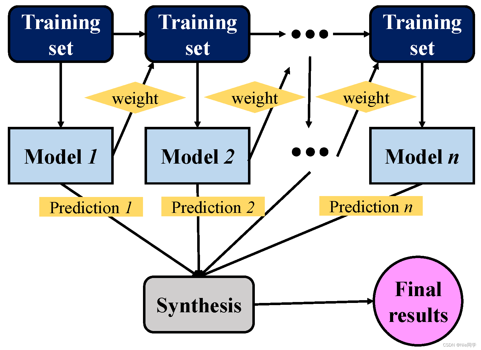
AdaBoost算法流程如下图所示：
在这里插入图片描述
下面我们采用基于加性模型的推导方式，即基学习器的线性组合：
$H(x)=\sum_{t=1}^T\alpha_th_t(x) \tag{1}$

其最小化指数损失函数为：
$\ell_{exp}(H|\mathcal{D})=\mathbb{E}_x\sim \mathcal{D}[e^{-f(x)H(x)}] \tag{2}$

即 $\mathcal{D}[e^{-f(x)H(x)}]$ 可以被理解为在分布 $\mathcal{D}$ 下，函数 $e^{-f(x)H(x)}$ 的期望值；其中 $f (x)$ 是真实值； $H (x)$ 为模型的预测值；

AdaBoost算法正确性说明

再此之前我们先把（2）式展开

对于离散型：
$\ell_{exp}(H|\mathcal{D})=\sum_x \mathcal{D}(x) e^{-f(x)H(x)} \tag{3}$
对于连续型：
$\ell_{exp}(H|\mathcal{D})=\int \mathcal{D}(x) e^{-f(x)H(x)}dx \tag{4}$

以离散型为例，接着使用最小二乘法，使得 $\ell_{exp}$ 最小，即对 $\ell_{exp}$ 求对 $H (x)$ 的偏导有：
$\begin{aligned} \frac{\partial \ell_{\text{exp}}(H|\mathcal{D})}{\partial H(x)} &= \sum_x \frac{\partial \mathcal{D}(x) e^{-f(x)H(x)}}{\partial H(x)} \\ &= \sum_x-\mathcal{D(x)}f(x)e^{-f(x)H(x)} \\ \end{aligned} \tag{5}$

又因为 $f(x)\in\{-1,+1\}$ ，所以式（5）可变形为：
$\begin{aligned} & \sum_x-\mathcal{D(x)}f(x)e^{-f(x)H(x)} \\ &= -\sum_x\mathcal{D}(x)e^{-H(x)}+\sum_x\mathcal{D}(x)e^{H(x)} \\ &= -e^{-H(x)} P(f(x)=1|x)+e^{H(x)}P(f(x)=-1|x) \end{aligned} \tag{6}$

其中 $P (f (x) = 1∣ x)$ 代表在数据集 $x$ 中好瓜的概率； $P (f (x) = - 1∣ x)$ 代表在数据集 $x$ 中坏瓜的概率。

令（6）式为零可得：
$H(x)=\frac{1}{2}\ln\frac{P(f(x)=1|x)}{P(f(x)=-1|x)} \tag{7}$

又因为对于一个二分类问题 $H(x)\in\{-1,+1\}$ ，故可将（7）式简化，有：
$\begin{aligned} \mathrm{sign}(H(x))&=\mathrm{sign}(\frac{1}{2}\ln\frac{P(f(x)=1|x)}{P(f(x)=-1|x)})\\ &=\begin{cases} 1,\quad P(f(x)=1|x)>P(f(x)=-1|x)\\ -1,\quad P(f(x)=1|x)<P(f(x)=-1|x) \end{cases}\\ &=\underset{y\in\{-1,+1\}}{\text{max}} \quad P(f(x)=y|x) \end{aligned} \tag{8}$

其中 $\underset{y\in\{-1,+1\}}{\text{max}} \quad P(f(x)=y|x)$ 该部分可以理解为在给定输入 $x$ 的情况下，选择具有最大条件概率的类别 $y$ ，即谁的概率大，就是什么类别。

这就意味着 $\mathrm{sign}(H(x))$ 达到了贝叶斯最优错误率。这说明指数损失函数是分类任务原本 $0/1$ 损失函数的一致性替代损失函数。因为该函数具有较好的数学性质，故用它来替代原本的 $0/1$ 损失函数是较好的选择。

AdaBoost算法如何解决权重更新问题？

在AdaBoost算法中，第一个基分类器 $h_1$ 是通过直接将基学习器算法用于初始数据分布而得到的；此后的每次迭代地生成 $h_t$ 和 $\alpha_t$ ，当基分类器 $h_t$ 基于分布 $\mathcal{D_t}$ 产生后，该分类器的权重应该使得 $\alpha_th_t$ 最小化指数损失函数
$\begin{aligned} \ell_{exp}(\alpha_th_t|\mathcal{D}_t)&=\mathbb{E}_x\sim \mathcal{D}_t[e^{-f(x)\alpha_th_t(x)}] \\ &= \sum_x\mathcal{D_t(x)}e^{-f(x)\alpha_th_t(x)} \\ \end{aligned} \tag{9}$

此时对于式（9）我们可以分类讨论： $f(x)=h_t(x)$ 和 $f(x)\ne h_t(x)$ ，有：
$\begin{aligned} & \sum_x\mathcal{D_t(x)}e^{-f(x)\alpha_th_t(x)} \\ &=e^{-\alpha_t}P(f(x)=h_t(x)|x)+e^{\alpha_t}P(f(x)\ne h_t(x)|x)\\ &=e^{-\alpha_t}P_x\sim\mathcal{D}_t[f(x)=h_t(x)]+e^{\alpha_t}P_x\sim\mathcal{D}_t[f(x)\ne h_t(x)]\\ &=e^{-\alpha_t}(1-\epsilon_t)+e^{\alpha_t}\epsilon_t \end{aligned} \tag{10}$
其中 $\epsilon_t=P_x\sim\mathcal{D}_t[f(x)\ne h_t(x)]$ ，考虑到指数损失函数对 $\alpha_t$ （权重）求偏导有：

$\frac{\partial \ell_{\text{exp}}(\alpha_th_t|\mathcal{D}_t)}{\partial \alpha_t}=-e^{-\alpha_t}(1-\epsilon_t)+e^{\alpha_t}\epsilon_t \tag{11}$

令式（11）为零有：
$\alpha_t=\frac{1}{2}\ln(\frac{1-\epsilon_t}{\epsilon_t}) \tag{12}$

这正是算法流程图中第六行的权重更新公式。

AdaBoost算法如何解决调整下一轮基学习器样本分布问题？

AdaBoost算法在获得 $H_{t-1}$ 之后的样本分布将进行调整，使得下一轮的基学习器 $h_t$ 能纠正 $H_{t-1}$ 的一些错误，理想的 $h_t$ 能纠正 $H_{t-1}$ 的全部错误，即最小化：

$\begin{aligned} \ell_{exp}(H_{t-1}+h_t|\mathcal{D})&=\mathbb{E}_x\sim \mathcal{D}[e^{-f(x)(H_{t-1}(x)+h_t(x))}] \\ &= \mathbb{E}_x\sim \mathcal{D}[e^{-f(x)H_{t-1}(x)}e^{-f(x)h_t(x)}] \\ \end{aligned} \tag{13}$

注意到 $f (x)$ 和 $h_t(x)\in\{-1,+1\}$ 故， $f^2(x)=h^2_t(x)=1$ ，因为 $e^x \approx 1 + x + \frac{x^2}{2!} + \frac{x^3}{3!} + \frac{x^4}{4!} + \ldots$ ；故可对式（13）中的 $e^{-f(x)h_t(x)}$ 泰勒展开近似为：
$\begin{aligned} \ell_{exp}(H_{t-1}+h_t|\mathcal{D})&\approx\mathbb{E}_x\sim \mathcal{D}[e^{-f(x)H_{t-1}(x)}(1-f(x)h_t(x))+\frac{f^2(x)h^2_t(x)}{2})] \\ &=\mathbb{E}_x\sim \mathcal{D}[e^{-f(x)H_{t-1}(x)}(1-f(x)h_t(x))+\frac{1}{2})] \end{aligned} \tag{14}$

于是，理想的基学习器
$\begin{aligned} h_t(x)&=\underset{h}{\text{arg min}} \quad \ell_{exp}(H_{t-1}+h|\mathcal{D}) \\ &=\underset{h}{\text{arg min}} \quad \mathbb{E}_x\sim \mathcal{D}[e^{-f(x)H_{t-1}(x)}(1-f(x)h(x))+\frac{1}{2})] \\ \end{aligned} \tag{15}$

因为式（15）中 $(1-f(x)h_t(x))+\frac{1}{2})$ $1$ 和 $\frac{1}{2}$ 与最终结果无关，故可以省略，且-号变为+号将目标函数从求最小变成求最大值，故式（15）可简化为：
$\begin{aligned} &\underset{h}{\text{arg min}} \quad \mathbb{E}_x\sim \mathcal{D}[e^{-f(x)H_{t-1}(x)}(1-f(x)h(x))+\frac{1}{2})] \\ &=\underset{h}{\text{arg max}} \quad \mathbb{E}_x\sim \mathcal{D}[e^{-f(x)H_{t-1}(x)}f(x)h(x)] \\ &=\underset{h}{\text{arg max}} \quad \mathbb{E}_x\sim \mathcal{D}[\frac{e^{-f(x)H_{t-1}(x)}}{\mathbb{E}_x\sim \mathcal{D}[e^{-f(x)H_{t-1}(x)}]}f(x)h(x)] \end{aligned}\tag{16}$

注意到 $\mathbb{E}_x\sim \mathcal{D}[e^{-f(x)H_{t-1}(x)}]$ 是一个常数。令 $\mathcal{D}_t$ 表示一个分布，使其更符合概率密度函数的定义：
$\mathcal{D_t}=\frac{\mathcal{D(x)}e^{-f(x)H_{t-1}(x)}}{\mathbb{E}_x\sim \mathcal{D}[e^{-f(x)H_{t-1}(x)}]} \tag{17}$

其中 $\mathcal{D_t}(x)$ 表示未来的分布函数， $D (x)$ 表示过去的分布函数。

根据数学期望的定义，等价于：
$\begin{aligned} h_t(x)&=\underset{h}{\text{arg max}} \quad \mathbb{E}_x\sim \mathcal{D}[\frac{e^{-f(x)H_{t-1}(x)}}{\mathbb{E}_x\sim \mathcal{D}[e^{-f(x)H_{t-1}(x)}]}f(x)h(x)]\\ &=\underset{h}{\text{arg max}} \quad \mathbb{E}_x\sim \mathcal{D_t}[f(x)h(x)] \end{aligned}\tag{18}$

由于 $f(x),h(x)\in \{-1,+1\}$ ，有：
$f(x)h(x)=1-2\chi{(f(x)\ne h(x))} \tag{19}$
其中 $\chi{(f(x)\ne h(x))}$ 的定义如下：
$\chi{(f(x) \ne h_t(x))} = \begin{cases} 1 & \text{如果 } f(x) \ne h(x) \\ 0 & \text{如果 } f(x) = h(x) \end{cases} \tag{20}$

则理想的基学习器为：
$h_t(x)=\underset{h}{\text{arg min}} \quad \mathbb{E}_x\sim \mathcal{D_t}[\chi(f(x)\ne h(x))] \tag{21}$

考虑到 $\mathcal{D_t}$ 与 $\mathcal{D_{t+1}}$ 的关系有：
$\begin{aligned} \mathcal{D_{t+1}}(x)&=\frac{\mathcal{D(x)}e^{-f(x)H_{t}(x)}}{\mathbb{E}_x\sim \mathcal{D}[e^{-f(x)H_{t}(x)}]} \\ &=\frac{\mathcal{D(x)}e^{-f(x)(H_{t-1}(x)+\alpha_th_t(x))}}{\mathbb{E}_x\sim \mathcal{D}[e^{-f(x)H_{t}(x)}]} \\ &= \frac{\mathcal{D(x)}e^{-f(x)H_{t-1}(x)}e^{-f(x)\alpha_th_t(x)}}{\mathbb{E}_x\sim \mathcal{D}[e^{-f(x)H_{t}(x)}]} \\ &=\frac{\mathcal{D(x)}e^{-f(x)H_{t-1}(x)}e^{-f(x)\alpha_th_t(x)}}{\mathbb{E}_x\sim \mathcal{D}[e^{-f(x)H_{t-1}(x)}]}\cdot \frac{\mathbb{E}_x\sim \mathcal{D}[e^{-f(x)H_{t-1}(x)}]}{\mathbb{E}_x\sim \mathcal{D}[e^{-f(x)H_{t}(x)}]}\\ &=\mathcal{D_t(x)} \cdot e^{-f(x)\alpha_th_t(x)}\frac{\mathbb{E}_x\sim \mathcal{D}[e^{-f(x)H_{t-1}(x)}]}{\mathbb{E}_x\sim \mathcal{D}[e^{-f(x)H_{t}(x)}]} \end{aligned} \tag{22}$

其中 $\frac{\mathbb{E}_x\sim \mathcal{D}[e^{-f(x)H_{t-1}(x)}]}{\mathbb{E}_x\sim \mathcal{D}[e^{-f(x)H_{t}(x)}]}$ 是常数。这就是AdaBoost算法流程图中第7行的样本分布更新公式。

AdaBoost算法总结

需要注意的是，AdaBoost算法对于无法接受带权样本的基学习算法，可通过重采样法来处理，即在每一轮学习中，根据样本分布对训练集进行重新采样，再用重采样而得到的样本集对基学习器进行训练。

偏差-方差分解是解释模型在预测中的性能时的一种常用方法。在这个角度来看，Boosting算法（例如AdaBoost）可以被解释为一个降低偏差并提高模型复杂度的方法。

偏差（Bias）： 表示模型的预测值与实际值的差异。高偏差意味着模型对训练数据的拟合不足。在Boosting中，通过迭代训练弱学习器，并对先前模型分类错误的样本进行更多关注，模型逐渐减小了偏差。每个弱学习器可能拟合不足，但通过组合它们，整个模型能够更好地适应训练数据。
方差（Variance）： 表示模型对训练数据的敏感性。高方差意味着模型对训练数据的小扰动很敏感，可能导致对新数据的泛化能力较差。Boosting通过降低弱学习器的方差来提高整个模型的泛化能力。每个弱学习器都是一个简单的模型，通常是一个深度较浅的决策树桩，因此具有较低的方差。

在Boosting中，每一轮迭代都会调整样本的权重，使得模型更加关注先前分类错误的样本。这种调整增加了模型对先前被错误分类的样本的拟合程度，降低了偏差。与此同时，通过使用多个弱学习器的组合，整体模型具有较低的方差，更有助于泛化到新数据。

总体而言，Boosting通过对高偏差、低方差的弱学习器的集成，实现了偏差-方差的权衡，提高了整体模型的性能和泛化能力。

实验分析

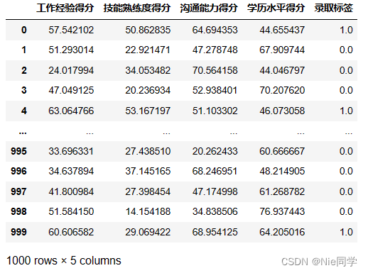
这个数据集包含了工作经验得分、技能熟练度得分、沟通能力得分、学历水平得分以及录取标签。我们的目标是利用工作经验、技能熟练度、沟通能力和学历等属性信息，通过机器学习模型来预测一个人是否被录取。

import pandas as pd
from sklearn.model_selection import train_test_split
from sklearn.ensemble import AdaBoostClassifier
from sklearn.tree import DecisionTreeClassifier
from sklearn.metrics import accuracy_score

# 读取数据
data = pd.read_csv('data/adaboost_recruitment_dataset_scores.csv')
data

在这里插入图片描述

# 分离特征和标签
X = data.drop('录取标签', axis=1)
y = data['录取标签']

# 将数据分为训练集和测试集
X_train, X_test, y_train, y_test = train_test_split(X, y, test_size=0.2, random_state=42)

用决策树算法

# 创建决策树分类器
decision_tree_clf = DecisionTreeClassifier(max_depth=1, random_state=42)

# 训练模型
decision_tree_clf.fit(X_train, y_train)

# 在测试集上进行预测
y_pred_decision_tree = decision_tree_clf.predict(X_test)

# 评估准确性
decision_tree_accuracy = accuracy_score(y_test, y_pred_decision_tree)
print(f'准确性: {
     decision_tree_accuracy:.2f}')

准确性: 0.87
用AdaBoost算法

# 创建 AdaBoostClassifier 的实例，使用决策树作为基分类器
base_classifier = DecisionTreeClassifier(max_depth=1)
adaboost_clf = AdaBoostClassifier(base_classifier, n_estimators=60, random_state=42)

# 训练模型
adaboost_clf.fit(X_train, y_train)

# 在测试集上进行预测
y_pred_adaboost = adaboost_clf.predict(X_test)

# 评估准确性
adaboost_accuracy = accuracy_score(y_test, y_pred_adaboost)
print(f'准确性: {
     adaboost_accuracy:.2f}')

准确性: 0.92
绘制评价图像

import matplotlib.pyplot as plt
import seaborn as sns
from sklearn.metrics import confusion_matrix, classification_report

plt.rcParams['font.sans-serif'] = ['SimHei']  # 设置中文字体为黑体
plt.rcParams['axes.unicode_minus'] = False  # 解决坐标轴负号'-'显示为方块的问题

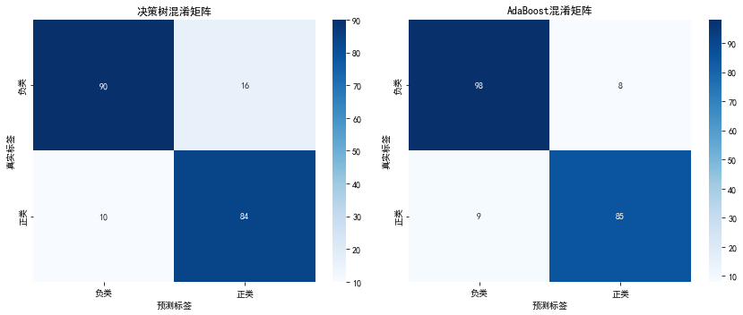
# 绘制单一决策树的混淆矩阵
conf_matrix_decision_tree = confusion_matrix(y_test, y_pred_decision_tree)
plt.figure(figsize=(12, 5))

plt.subplot(1, 2, 1)
sns.heatmap(conf_matrix_decision_tree, annot=True, fmt='d', cmap='Blues', xticklabels=['负类', '正类'], yticklabels=['负类', '正类'])
plt.xlabel('预测标签')
plt.ylabel('真实标签')
plt.title('决策树混淆矩阵')

# 绘制 AdaBoost 的混淆矩阵
conf_matrix_adaboost = confusion_matrix(y_test, y_pred_adaboost)

plt.subplot(1, 2, 2)
sns.heatmap(conf_matrix_adaboost, annot=True, fmt='d', cmap='Blues', xticklabels=['负类', '正类'], yticklabels=['负类', '正类'])
plt.xlabel('预测标签')
plt.ylabel('真实标签')
plt.title('AdaBoost混淆矩阵')

plt.tight_layout()
plt.show()

# 打印单一决策树的分类报告
print("单一决策树分类报告：\n", classification_report(y_test, y_pred_decision_tree))

# 打印 AdaBoost 的分类报告
print("AdaBoost分类报告：\n", classification_report(y_test, y_pred_adaboost))

在这里插入图片描述

单一决策树分类报告：
               precision    recall  f1-score   support

         0.0       0.90      0.85      0.87       106
         1.0       0.84      0.89      0.87        94

    accuracy                           0.87       200
   macro avg       0.87      0.87      0.87       200
weighted avg       0.87      0.87      0.87       200

AdaBoost分类报告：
               precision    recall  f1-score   support

         0.0       0.92      0.92      0.92       106
         1.0       0.91      0.90      0.91        94

    accuracy                           0.92       200
   macro avg       0.91      0.91      0.91       200
weighted avg       0.91      0.92      0.91       200

根据上述分析报告，可知AdaBoost模型相对于单一决策树表现更佳，具有更高的准确度和综合指标。在AdaBoost中，对未被录取和被录取的预测精确性较高，同时识别实际样本的能力也表现出色，呈现出更好的泛化性能。