1.Radar图简介
最近在数学建模中碰见需要绘制Radar图(雷达图)的情况来具体分析样本的各个特征之间的得分与优劣关系,这样的情况比较符合雷达图的使用场景,一般来说,雷达图适用于展示多个维度的数据,并在一个平面上直观地呈现出不同维度的变化趋势,比较适用的场合如下:
∙ \bullet ∙综合评价: 雷达图是理想的工具,能够直观展示多个评价指标的得分,为综合评估提供清晰的整体表现概览。
∙ \bullet ∙SWOT分析: 通过SWOT分析,雷达图展示了组织或项目在各方面的优势、劣势、机会和威胁,为战略决策提供直观支持。
∙ \bullet ∙个体特征对比: 通过雷达图,我们可以比较不同个体在各个特征上的差异,无论是个人技能评估还是产品性能对比,一目了然。
2.Radar图绘图案例:单样本图绘制
import numpy as np
import matplotlib.pyplot as plt
import matplotlib
import warnings
warnings.filterwarnings("ignore")
matplotlib.rcParams['font.family'] = 'serif'
matplotlib.rcParams['font.serif'] = 'Times New Roman'
#需要评价的特征名称
labels = np.array(['Comprehensive', 'Education', 'Professional Title', 'Teaching', 'Training', 'Research'])
labels = np.array(['A1', 'A2', 'A3', 'A4', 'A5', 'A6'])
#需要评价的特征的数量
nAttr = len(labels)
#数据/得分情况
data = np.array([8, 5, 8, 9, 8, 6])
#计算角度360/n
angels = np.linspace(0, 2*np.pi, nAttr, endpoint=False)
#创建数据闭环效果
data = np.concatenate((data, [data[0]]))
angels = np.concatenate((angels, [angels[0]]))


#可视化绘图
fig = plt.figure(facecolor='white')
ax = plt.subplot(111, polar=True)

ax.set_ylim(0, 10)
#绘制线条
ax.plot(angels, data, 'o-', color='lightgreen', linewidth=2, label='A Personal Characteristics')

#添加数值标签(选写)
for i in range(len(angels)-1):
    ax.text(angels[i], data[i]+0.8, str(data[i]), color='b')

#填充区域
ax.fill(angels, data, facecolor='red', alpha=0.25)
ax.set_xticks(angels[:-1])
ax.set_xticklabels(labels, ha='center')
ax.set_title('Academic Scholar Research Feature Radar Chart', va='bottom', fontweight='bold')
#设置一些图例要求
plt.grid(True)
#plt.legend(loc='upper right')
#plt.legend(loc='upper right', bbox_to_anchor=(1.2, 0.55), bbox_transform=plt.gcf().transFigure)
plt.savefig('雷达图1.jpg')
plt.show()

3.Radar图绘图案例:多样本图绘制
import numpy as np
import matplotlib.pyplot as plt
import matplotlib
import warnings

warnings.filterwarnings("ignore")

matplotlib.rcParams['font.family'] = 'serif'
matplotlib.rcParams['font.serif'] = 'Times New Roman'
matplotlib.rcParams['font.style'] = 'italic'

radar_labels = np.array(['A1', 'A2', 'A3',
                         'A4', 'A5', 'A6'])
nAttr = 6

data = np.array([[0.40, 0.32, 0.35, 0.30, 0.30, 0.88],
                 [0.85, 0.35, 0.30, 0.40, 0.40, 0.30],
                 [0.43, 0.89, 0.30, 0.28, 0.22, 0.30],
                 [0.30, 0.25, 0.48, 0.85, 0.45, 0.40],
                 [0.20, 0.38, 0.87, 0.45, 0.32, 0.28],
                 [0.34, 0.31, 0.38, 0.40, 0.92, 0.28]])
data_labels = ('Engineer', 'Laboratory Technician', 'Artist', 'Salesperson', 'Social Worker', 'Clerk')

angles = np.linspace(0, 2*np.pi, nAttr, endpoint=False)

data = np.concatenate((data, [data[0]]))
angles = np.concatenate((angles, [angles[0]]))

fig = plt.figure(facecolor='white')
ax = plt.subplot(111, polar=True)

ax.plot(angles, data, 'o-', linewidth=1, alpha=0.2)
ax.fill(angles, data, alpha=0.3)

ax.set_thetagrids(np.degrees(angles[0:6]), labels=radar_labels)
ax.set_title('Holland Personality Analysis', va='bottom', fontweight='bold', size=16)

legend = plt.legend(data_labels, loc=(1.1, 0.55), labelspacing=0.1, edgecolor='k', fontsize=10)

plt.grid(True)
plt.savefig('雷达图2.jpg')
plt.show()

4.Radar图绘图案例:Matplotlib标准绘图案例
import numpy as np
import matplotlib.pyplot as plt
from matplotlib.patches import Circle, RegularPolygon
from matplotlib.path import Path
from matplotlib.projections.polar import PolarAxes
from matplotlib.projections import register_projection
from matplotlib.spines import Spine
from matplotlib.transforms import Affine2D


def radar_factory(num_vars, frame='circle'):
    """
    Create a radar chart with `num_vars` axes.

    This function creates a RadarAxes projection and registers it.

    Parameters
    ----------
    num_vars : int
        Number of variables for radar chart.
    frame : {'circle', 'polygon'}
        Shape of frame surrounding axes.

    """
    # calculate evenly-spaced axis angles
    theta = np.linspace(0, 2*np.pi, num_vars, endpoint=False)

    class RadarTransform(PolarAxes.PolarTransform):

        def transform_path_non_affine(self, path):
            # Paths with non-unit interpolation steps correspond to gridlines,
            # in which case we force interpolation (to defeat PolarTransform's
            # autoconversion to circular arcs).
            if path._interpolation_steps > 1:
                path = path.interpolated(num_vars)
            return Path(self.transform(path.vertices), path.codes)

    class RadarAxes(PolarAxes):

        name = 'radar'
        PolarTransform = RadarTransform

        def __init__(self, *args, **kwargs):
            super().__init__(*args, **kwargs)
            # rotate plot such that the first axis is at the top
            self.set_theta_zero_location('N')

        def fill(self, *args, closed=True, **kwargs):
            """Override fill so that line is closed by default"""
            return super().fill(closed=closed, *args, **kwargs)

        def plot(self, *args, **kwargs):
            """Override plot so that line is closed by default"""
            lines = super().plot(*args, **kwargs)
            for line in lines:
                self._close_line(line)

        def _close_line(self, line):
            x, y = line.get_data()
            # FIXME: markers at x[0], y[0] get doubled-up
            if x[0] != x[-1]:
                x = np.append(x, x[0])
                y = np.append(y, y[0])
                line.set_data(x, y)

        def set_varlabels(self, labels):
            self.set_thetagrids(np.degrees(theta), labels)

        def _gen_axes_patch(self):
            # The Axes patch must be centered at (0.5, 0.5) and of radius 0.5
            # in axes coordinates.
            if frame == 'circle':
                return Circle((0.5, 0.5), 0.5)
            elif frame == 'polygon':
                return RegularPolygon((0.5, 0.5), num_vars,
                                      radius=.5, edgecolor="k")
            else:
                raise ValueError("Unknown value for 'frame': %s" % frame)

        def _gen_axes_spines(self):
            if frame == 'circle':
                return super()._gen_axes_spines()
            elif frame == 'polygon':
                # spine_type must be 'left'/'right'/'top'/'bottom'/'circle'.
                spine = Spine(axes=self,
                              spine_type='circle',
                              path=Path.unit_regular_polygon(num_vars))
                # unit_regular_polygon gives a polygon of radius 1 centered at
                # (0, 0) but we want a polygon of radius 0.5 centered at (0.5,
                # 0.5) in axes coordinates.
                spine.set_transform(Affine2D().scale(.5).translate(.5, .5)
                                    + self.transAxes)
                return {
   'polar': spine}
            else:
                raise ValueError("Unknown value for 'frame': %s" % frame)

    register_projection(RadarAxes)
    return theta


def example_data():
    # The following data is from the Denver Aerosol Sources and Health study.
    # See doi:10.1016/j.atmosenv.2008.12.017
    #
    # The data are pollution source profile estimates for five modeled
    # pollution sources (e.g., cars, wood-burning, etc) that emit 7-9 chemical
    # species. The radar charts are experimented with here to see if we can
    # nicely visualize how the modeled source profiles change across four
    # scenarios:
    #  1) No gas-phase species present, just seven particulate counts on
    #     Sulfate
    #     Nitrate
    #     Elemental Carbon (EC)
    #     Organic Carbon fraction 1 (OC)
    #     Organic Carbon fraction 2 (OC2)
    #     Organic Carbon fraction 3 (OC3)
    #     Pyrolyzed Organic Carbon (OP)
    #  2)Inclusion of gas-phase specie carbon monoxide (CO)
    #  3)Inclusion of gas-phase specie ozone (O3).
    #  4)Inclusion of both gas-phase species is present...
    data = [
        ['Sulfate', 'Nitrate', 'EC', 'OC1', 'OC2', 'OC3', 'OP', 'CO', 'O3'],
        ('Basecase', [
            [0.88, 0.01, 0.03, 0.03, 0.00, 0.06, 0.01, 0.00, 0.00],
            [0.07, 0.95, 0.04, 0.05, 0.00, 0.02, 0.01, 0.00, 0.00],
            [0.01, 0.02, 0.85, 0.19, 0.05, 0.10, 0.00, 0.00, 0.00],
            [0.02, 0.01, 0.07, 0.01, 0.21, 0.12, 0.98, 0.00, 0.00],
            [0.01, 0.01, 0.02, 0.71, 0.74, 0.70, 0.00, 0.00, 0.00]]),
        ('With CO', [
            [0.88, 0.02, 0.02, 0.02, 0.00, 0.05, 0.00, 0.05, 0.00],
            [0.08, 0.94, 0.04, 0.02, 0.00, 0.01, 0.12, 0.04, 0.00],
            [0.01, 0.01, 0.79, 0.10, 0.00, 0.05, 0.00, 0.31, 0.00],
            [0.00, 0.02, 0.03, 0.38, 0.31, 0.31, 0.00, 0.59, 0.00],
            [0.02, 0.02, 0.11, 0.47, 0.69, 0.58, 0.88, 0.00, 0.00]]),
        ('With O3', [
            [0.89, 0.01, 0.07, 0.00, 0.00, 0.05, 0.00, 0.00, 0.03],
            [0.07, 0.95, 0.05, 0.04, 0.00, 0.02, 0.12, 0.00, 0.00],
            [0.01, 0.02, 0.86, 0.27, 0.16, 0.19, 0.00, 0.00, 0.00],
            [0.01, 0.03, 0.00, 0.32, 0.29, 0.27, 0.00, 0.00, 0.95],
            [0.02, 0.00, 0.03, 0.37, 0.56, 0.47, 0.87, 0.00, 0.00]]),
        ('CO & O3', [
            [0.87, 0.01, 0.08, 0.00, 0.00, 0.04, 0.00, 0.00, 0.01],
            [0.09, 0.95, 0.02, 0.03, 0.00, 0.01, 0.13, 0.06, 0.00],
            [0.01, 0.02, 0.71, 0.24, 0.13, 0.16, 0.00, 0.50, 0.00],
            [0.01, 0.03, 0.00, 0.28, 0.24, 0.23, 0.00, 0.44, 0.88],
            [0.02, 0.00, 0.18, 0.45, 0.64, 0.55, 0.86, 0.00, 0.16]])
    ]
    return data


if __name__ == '__main__':
    N = 9
    theta = radar_factory(N, frame='polygon')

    data = example_data()
    spoke_labels = data.pop(0)

    fig, axs = plt.subplots(figsize=(9, 9), nrows=2, ncols=2,
                            subplot_kw=dict(projection='radar'))
    fig.subplots_adjust(wspace=0.25, hspace=0.20, top=0.85, bottom=0.05)

    colors = ['b', 'r', 'g', 'm', 'y']
    # Plot the four cases from the example data on separate axes
    for ax, (title, case_data) in zip(axs.flat, data):
        ax.set_rgrids([0.2, 0.4, 0.6, 0.8])
        ax.set_title(title, weight='bold', size='medium', position=(0.5, 1.1),
                     horizontalalignment='center', verticalalignment='center')
        for d, color in zip(case_data, colors):
            ax.plot(theta, d, color=color)
            ax.fill(theta, d, facecolor=color, alpha=0.25, label='_nolegend_')
        ax.set_varlabels(spoke_labels)

    # add legend relative to top-left plot
    labels = ('Factor 1', 'Factor 2', 'Factor 3', 'Factor 4', 'Factor 5')
    legend = axs[0, 0].legend(labels, loc=(0.98, -0.2),
                              labelspacing=0.1, fontsize=12,edgecolor='k')

    fig.text(0.5, 0.965, '5-Factor Solution Profiles Across Four Scenarios',
             horizontalalignment='center', color='black', weight='bold',
             size=16)
    plt.savefig('雷达图3.jpg')
    plt.show()