一、说明
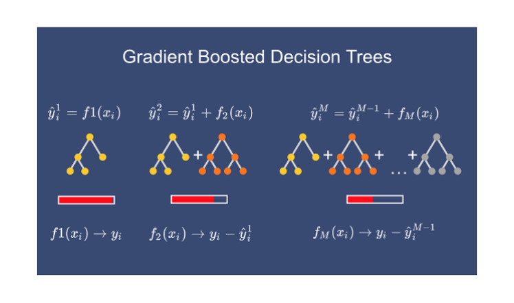
在在这篇文章中,我们学习了另一种称为梯度增强的集成技术。这是我在机器学习算法集成技术文章系列中与bagging一起介绍的一种增强技术。我还讨论了随机森林和 AdaBoost 算法。但在这里我们讨论的是梯度提升,在我们深入研究梯度提升之前,了解决策树很重要。因此,如果您不熟悉决策树,那么理解梯度提升可能并不容易。请参阅本文以更好地了解决策树。
二、建立模型
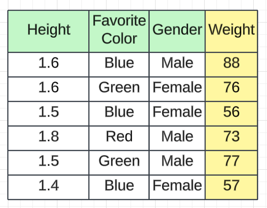
我们以身高、最喜欢的颜色、性别作为独立特征,体重作为输出特征的数据集为例。我们有 6 条记录。
2.1 步骤1:
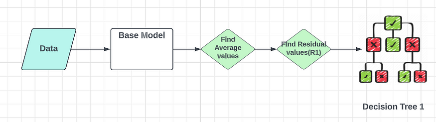
决策树的第一步是计算基本模型,它是所有权重的平均值。
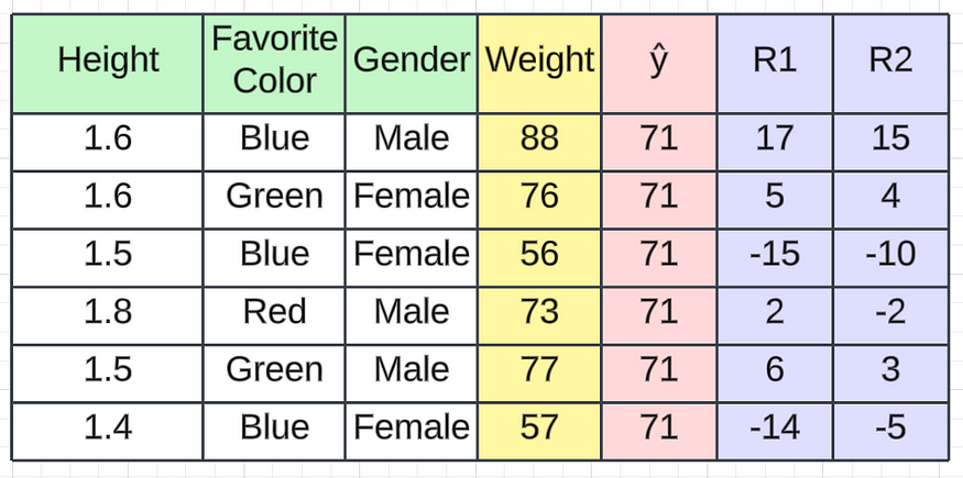
Average Salary(ŷ) = (88 + 76 + 56 + 73 + 77 + 57)/ 6 = 71.17 ≈ 71当我们给出训练数据集时,预测值为71.17。这只是我们计算的平均工资。为了更好的解释,我们将其用作≈71 。
2.2 第2步:
在第二步中,我们将计算残差,也称为伪残差。在回归中,我们使用损失函数来计算误差。有不同的损失函数,例如均方误差、回归和对数损失的均方根误差以及分类的铰链损失。根据所选的损失函数,我们将计算残差。在这种情况下,我们将使用一个简单的损失函数。损失将通过从预测值中减去实际值来计算(例如,我们使用此计算),从而产生一个名为R1的新列,表示残差。
例如,如果我们从 88 中减去 71 ,则第一条记录的残差将为17。

2.3 步骤3:
建立好这个基础模型后,我们将依次添加一棵决策树。在这个决策树中,我的输入是身高、最喜欢的颜色和性别。我的依赖特征不是重量。这将是残余误差 R1。基于此我们可以创建决策树。
现在我们有了一个基本模型和一个决策树。我们已经训练了决策树。当我们将新数据传递给决策树时,它将预测残差值的输出。我们将其命名为残差 2(R2)输出。

在此基础上,让我们检查一下预测的进展情况。假设我们得到这样的 R2 值。
R2 值
因此,每当我们通过基本模型获取第一条记录时,它将是71(我们计算的平均值)。转到决策树 1,我们将获得一些残差值。从上图中,您可以看到我们获得的第一条记录的残差值(R2)为 15 。如果我们将其与 71 相加,我们将得到一个值86,该值非常接近实际值。
1st Record
==================
R1 = 15
Average Weight = 71
Predicted Weight = 71 + 15 = 86然而,这凸显了决策树模型中的过度拟合问题。我们想要创建一个具有低方差和低偏差的通用模型。在这种情况下,我们的偏差较低,但方差较高,这意味着当引入新的测试数据时,该值可能会下降。为了解决这个问题,我们将向模型添加学习率Alpha (α)和 R2 值。学习率应该在 0 到 1 之间。
Assume α = 0.1
Predicted Weight  = Avearge Weight + α (R2 Value)
= 71 + (0.1)15 = 72.5在这里您可以看到72.5,这与实际重量存在显着差异。将根据残差 2(R2) 值和相同的独立特征添加额外的决策树来解决此问题。该决策树将依次计算我的下一个残差。通用公式可以写成:
F(x) = h0x + α1 h1x + α2 h2x + α3 h3x + ....... + αn hnx

F(x) = i = 1 -> n Σ αi hix

h0x = Base Model
hnxn = Output given by any desicion tree目标是通过根据残差顺序创建决策树来减少残差。Alpha(α)次要参数将使用次要参数调整来决定。

基本上,在基本模型之后,我们会依次使用决策树来增强模型。这就是为什么它被称为增强技术。
三、该算法背后的伪代码
现在我们将深入研究我们创建的伪算法背后的数学原理。尽管看起来很复杂,但我们将分解每个步骤以帮助您理解该过程。我们使用的数据集包括身高、喜欢的颜色、性别和体重,共有 6 条记录。身高、喜欢的颜色和性别是我的独立特征,体重是我的从属特征。
3.1 遵循伪算法所需的基本步骤
- 提供输入——独立和相关特征。
- 提供损失函数——这对于分类问题(对数损失和铰链损失)或回归问题(均方误差、均方根误差)可能有所不同。所有的损失函数应该是可微的(能够求导数)。
- 找出梯度提升算法中需要多少棵树。
3.2 计算步骤
3.2.1 步骤1 -
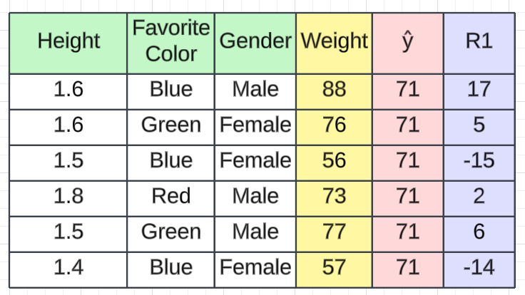
梯度提升的第一步是构建一个基础模型来预测训练数据集中的观察结果。为简单起见,我们取目标列 (ŷ) 的平均值,并假设其为预测值,如红色列下方所示。

为什么我说我们取目标列的平均值?嗯,这涉及到数学。从数学上讲,第一步可以写为:

---------------------------------------------
F0(x) = arg min γ (i = 1 -> n Σ Loss(y,γ))
---------------------------------------------

L      = loss function
γ      = predicted value
argmin = we have to find a predicted value/γ for which the loss function is minimum.

Loss Function (Regresion)
==========================
Loss  = [i = 0 -> n Σ 1/n (yi - γi)²]

yi     = observed value (weight)
γ      = predicted value

// Now we need to find a minimum value of γ such that this loss function is minimum.
// We use to differentiate this loss function and then put it equal to 0 right? Yes, we will do the same here.
d(Loss)/ dγ = d([i = 0 -> n Σ 1/n (yi - γi)²])/ dγ
d(Loss)/ dγ = 2/2(i = 0 -> n Σ (yi - γi)) * (-1) = - (i = 0 -> n Σ (yi - γi)) - equation 1

// Let’s see how to do this with the help of our example.
// Remember that yi is our observed value and γi is our predicted value, by plugging the values in the above formula we get:
d(Loss)/ dγ = - [88 - γ + 76 - γ + 56 - + 73 - γ + 77 - γ + 57 - γ]
            = - 427 + 6γ

d(Loss)/ dγ = 0
- 427 + 6γ  = 0
6γ          = 427
γ           = 71.16 ≈ 71

// We end up over an average of the observed weight and this is why I asked you to take the average of the target column and assume it to be your first prediction.

Hence for γ=71, the loss function will be minimum so this value will become our prediction for the base model.
==============================================================================================================
3.2.2 第2步-
下一步是计算伪残差,即(观测值 - 预测值)。图中R1是计算出的残值。
问题又来了,为什么只是观察到预测?一切都有数学证明,我们看看这个公式从何而来。这一步可以写成:

----------------------------------
rim = - [dL(y1, F(x1)) / dF(x1)]
----------------------------------

F(xi) = previous model output
m     = number of DT made

// From the equation 1 We are just taking the derivative of loss function
d(Loss)/ dγ = - (i = 0 -> n Σ (yi - γi)) = -(i = 0 -> n Σ (Observed - Predicted))

// If you see the formula of residuals above, we see that the derivative of the loss function is multiplied by a negative sign, so now we get:
Observed - Predicted
// The predicted value here is the prediction made by the previous model.
// In our example the prediction made by the previous model (initial base model prediction) is 71, to calculate the residuals our formula becomes:
(Observed - 71)

Finding the rim values for the dataset
-----------------------------------------
r11 = 1st Record of model 1 = (y - ŷ) = 88 - 71 = 17
r21 = 2nd Record of model 1 = (y - ŷ) = 76 - 71 = 5
r31 = 3rd Record of model 1 = (y - ŷ) = 56 - 71 = -15
r41 = 4th Record of model 1 = (y - ŷ) = 73 - 71 = 2
r51 = 5th Record of model 1 = (y - ŷ) = 77 - 71 = 6
r61 = 6th Record of model 1 = (y - ŷ) = 57 - 71 = -14
3.2.3 步骤3—
下一步,我们将根据这些伪残差建立模型并进行预测。我们为什么要做这个?
因为我们希望最小化这些残差,最小化残差最终将提高我们的模型准确性和预测能力。因此,使用残差作为目标和原始特征高度、最喜欢的颜色和性别,我们将生成新的预测。请注意,在这种情况下,预测将是错误值,而不是预测的权重,因为我们的目标列现在是错误的(R1)。
3.2.4 步骤4 -
在此步骤中,我们找到决策树每个叶子的输出值。这意味着可能存在1 个叶子获得超过 1 个残差的情况,因此我们需要找到所有叶子的最终输出。为了找到输出,我们可以简单地取叶子中所有数字的平均值,无论只有 1 个数字还是多于 1 个数字。
让我们看看为什么我们要取所有数字的平均值。从数学上讲,该步骤可以表示为:

-----------------------------------------------
γm = argmin γ [i = 1 -> n Σ L(y1, Fm-1(x1) + γhm(xi))]
-------------------------------------------------

hm(xi) = DT made on residuals
m      = number of DT
γm     = output value of a particular leaf

// m = 1 we are talking about the 1st DT and when it is “M” we are talking about the last DT.
// The output value for the leaf is the value of γ that minimizes the Loss function

[Fm-1(xi)+ γhm(xi))] = This is similar as step 1 equation but here the difference is that we are taking previous predictions whereas earlier there was no previous prediction.

Let’s understand this even better with the help of an example. Suppose this is our regressor tree:


                 Height(> 1.5)
                /            \
               /              \
              /                \
          Fav Clr               Gender
            / \                    / \
           /   \                  /   \
          /     \                /     \
       R1,1     R2,1           R3,1    R4,1
      17        5, 2           -15    6, -14

γm = argmin γ [i = 1 -> n Σ L(y1, Fm-1(x1) + γhm(xi))]
// Using lost function we can write this as,
L(y1, Fm-1(x1) + γhm(xi) = 1/2 (y1 - (Fm-1(x1) + γhm(xi)))^2
Then,
γm = argmin γ [i = 1 -> n Σ 1/2 (y1 - (Fm-1(x1) + γhm(xi)))^2]

Let's see 1st residual goes in R1,1
γ1,1 = argmin 1/2(80 - (71 + γ))^2

//Now we need to find the value for γ for which this function is minimum.
// So we find the derivative of this equation w.r.t γ and put it equal to 0.
d (γ1,1) / d γ = d (1/2(88 - (71 + γ))^2) / dγ
0              = d (1/2(88 - (71 + γ))^2) / dγ
80 - (71 + γ)  = 0
γ              = 17


Let's see 1st residual goes in R2,1
γ2,1 = argmin 1/2(76 - (71 + γ))^2  +  1/2(73 - (71 + γ))^2

//Now we need to find the value for γ for which this function is minimum.
// So we find the derivative of this equation w.r.t γ and put it equal to 0.
d (γ2,1) / d γ = d (1/2(76 - (71 + γ))^2  +  1/2(73 - (71 + γ))^2) / dγ
0              = d (1/2(76 - (71 + γ))^2  +  1/2(73 - (71 + γ))^2) / dγ
-2γ + 5 + 2    = 0
γ              =  7 /2 = 3.5


Let's see 1st residual goes in R3,1
γ3,1 = argmin 1/2(56 - (71 + γ))^2

//Now we need to find the value for γ for which this function is minimum.
// So we find the derivative of this equation w.r.t γ and put it equal to 0.
d (γ3,1) / d γ = d (1/2(56 - (71 + γ))^2) / dγ
0              = d (1/2(56 - (71 + γ))^2) / dγ
-γ - 15        = 0
γ              = -15


Let's see 1st residual goes in R4,1
γ4,1 = argmin 1/2(77 - (71 + γ))^2  +  1/2(57 - (71 + γ))^2

//Now we need to find the value for γ for which this function is minimum.
// So we find the derivative of this equation w.r.t γ and put it equal to 0.
d (γ4,1) / d γ = d (1/2(77 - (71 + γ))^2  +  1/2(57 - (71 + γ))^2) / dγ
0              = d (1/2(77 - (71 + γ))^2  +  1/2(57 - (71 + γ))^2) / dγ
-2γ + 6 -14    = 0
γ              =  -8/2 = -4


// We end up with the average of the residuals in the leaf R2,1 and R4,1. Hence if we get any leaf with more than 1 residual, we can simply find the average of that leaf and that will be our final output.
现在计算所有叶子的输出后,我们得到,

3.2.5 步骤 5 —
这最终是我们必须更新先前模型的预测的最后一步。它可以更新为:
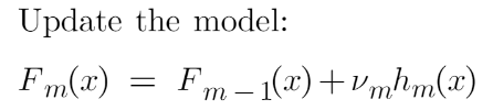
---------------------------
Fm(x) = Fm-1(x) + vmhm(x)
---------------------------
m       = number of decision trees made
Fm-1(x) = prediction of the base model (previous prediction)
Hm(x)   = recent DT made on the residuals

// since F1-1= 0 , F0 is our base model hence the previous prediction is 71.
vm is the learning rate that is usually selected between 0-1. It reduces the effect each tree has on the final prediction, and this improves accuracy in the long run. Let’s take vm=0.1 in this example.

Let’s calculate the new prediction now:

New Prediction F1(x) = 71 + 0.1 * Height(> 1.5)
                                 /            \
                                /              \
                               /                \
                           Fav Clr               Gender
                             / \                    / \
                            /   \                  /   \
                           /     \                /     \
                        R1,1     R2,1           R3,1    R4,1
                       17        5, 2           -15    6, -14
假设我们想要找到高度为 1.7 的第一个数据点的预测。这个数据点将经过这个决策树,它得到的输出将乘以学习率,然后添加到之前的预测中。
现在,更新预测后,我们需要再次迭代步骤 2 中的步骤以找到另一个决策树。这种情况将会发生,直到我们通过基于残差顺序创建决策树来减少残差。
现在假设m=2,这意味着我们已经构建了 2 个决策树,现在我们想要有新的预测。
这次我们将把之前的预测F1(x)添加到对残差进行的新 DT 中。我们将一次又一次地迭代这些步骤,直到损失可以忽略不计。
New Prediction F2(x) = 71 + (0.1 * DT value) + (0.1 * DT value)这就是梯度提升算法的全部内容。我希望您对这个主题有更好的理解。我们下一篇文章讨论XgBoost算法。