import numpy as np
import pandas as pd
import matplotlib.pyplot as plt
import seaborn as sns

plt.rcParams.update({'font.size': 20})
In [2]:
weather_data = pd.read_csv("../data/3/Summary of Weather.csv")
c:\users\skd621\anaconda3\lib\site-packages\IPython\core\interactiveshell.py:3020: DtypeWarning: Columns (7,8,18,25) have mixed types. Specify dtype option on import or set low_memory=False.
  interactivity=interactivity, compiler=compiler, result=result)
In [3]:
weather_data = weather_data.loc[:,["STA","Date","MeanTemp"]]
In [4]:
weather_data.head()
Out[4]:
| STA | Date | MeanTemp | |
|---|---|---|---|
| 0 | 10001 | 1942-7-1 | 23.888889 |
| 1 | 10001 | 1942-7-2 | 25.555556 |
| 2 | 10001 | 1942-7-3 | 24.444444 |
| 3 | 10001 | 1942-7-4 | 24.444444 |
| 4 | 10001 | 1942-7-5 | 24.444444 |
In [5]:
weather_data.info()
<class 'pandas.core.frame.DataFrame'>
RangeIndex: 119040 entries, 0 to 119039
Data columns (total 3 columns):
STA         119040 non-null int64
Date        119040 non-null object
MeanTemp    119040 non-null float64
dtypes: float64(1), int64(1), object(1)
memory usage: 2.7+ MB
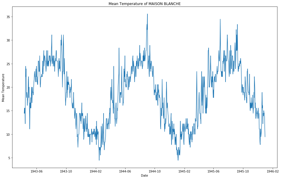
选择一个气象站,分析其温度变化的时间特性
In [6]:
weather_palmyra = weather_data[weather_data.STA == 33023]
weather_palmyra['Date'] = pd.to_datetime(weather_palmyra['Date'])
plt.figure(figsize=(16,10))
plt.plot(weather_palmyra.Date,weather_palmyra.MeanTemp)
plt.title("Mean Temperature of MAISON BLANCHE")
plt.xlabel("Date")
plt.ylabel("Mean Temperature")
plt.show()
c:\users\skd621\anaconda3\lib\site-packages\ipykernel_launcher.py:2: SettingWithCopyWarning:
A value is trying to be set on a copy of a slice from a DataFrame.
Try using .loc[row_indexer,col_indexer] = value instead

See the caveats in the documentation: http://pandas.pydata.org/pandas-docs/stable/indexing.html#indexing-view-versus-copy
In [7]:
timeSeries = weather_palmyra.loc[:, ["Date","MeanTemp"]]
timeSeries.index = timeSeries.Date
timeSeries = timeSeries.drop("Date",axis=1)
In [21]:
rolmean = timeSeries.rolling(6).mean()
rolstd = timeSeries.rolling(6).std()
plt.figure(figsize=(22,10))
orig = plt.plot(timeSeries, 'r-',label='Original')
mean = plt.plot(rolmean, 'b', label='Rolling Mean',marker='+', markersize=12)
std = plt.plot(rolstd, 'g--', label = 'Rolling Std')
plt.xlabel("Date")
plt.ylabel("Mean Temperature")
plt.title('Rolling Mean & Standard Deviation')
plt.legend()
plt.show()

In [22]:
from statsmodels.tsa.stattools import adfuller
# res = adfuller(timeSeries.MeanTemp)
res = adfuller(timeSeries.MeanTemp, autolag='AIC')
print('Test statistic: %.4f; p-value: %.4f'%(res[0], res[1]))
print("Critical Values: ",res[4])
Test statistic: -1.9031; p-value: 0.3306
Critical Values:  {'1%': -3.4369994990319355, '5%': -2.8644757356011743, '10%': -2.5683331327427803}
c:\users\skd621\anaconda3\lib\site-packages\statsmodels\compat\pandas.py:56: FutureWarning: The pandas.core.datetools module is deprecated and will be removed in a future version. Please use the pandas.tseries module instead.
  from pandas.core import datetools
In [34]:
def check_DF(timeSeries):
    res = adfuller(timeSeries.MeanTemp, autolag='AIC')
    print('Test statistic:%.4f;p-value: %.4f'%(res[0],res[1]))
    print("Critical Values: ",res[4])
def check_mean_std(timeSeries):
    rolmean = timeSeries.rolling(6).mean()
    rolstd = timeSeries.rolling(6).std()
    plt.figure(figsize=(22,10))
    orig = plt.plot(timeSeries, 'r-',label='Original')
    mean = plt.plot(rolmean, 'b', label='Rolling Mean',marker='+', markersize=10)
    std = plt.plot(rolstd, 'g', label = 'Rolling Std',marker='o', markersize=3)
    plt.xlabel("Date")
    plt.ylabel("Mean Temperature")
    plt.title('Rolling Mean & Standard Deviation')
    plt.legend()
    plt.show()
In [25]:
timeSeries_diff = timeSeries - timeSeries.shift(periods=1)
In [26]:
plt.figure(figsize=(16,12))
plt.plot(timeSeries_diff)
plt.title("Differencing method")
plt.xlabel("Date")
plt.ylabel("Differencing Mean Temperature")
plt.show()

In [27]:
timeSeries_diff.dropna(inplace=True)
In [28]:
check_DF(timeSeries_diff)
Test statistic:-15.4648;p-value: 0.0000
Critical Values:  {'1%': -3.4369994990319355, '5%': -2.8644757356011743, '10%': -2.5683331327427803}
In [35]:
check_mean_std(timeSeries_diff)

In [38]:
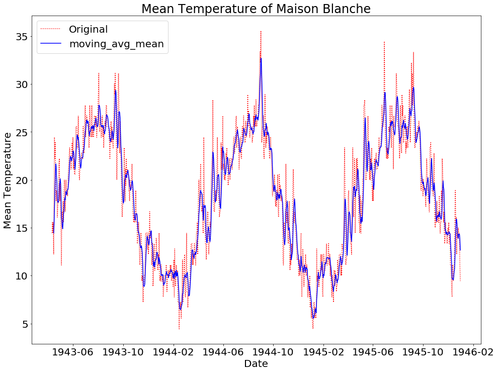
timeSeries_moving_avg = timeSeries.rolling(5).mean()
In [47]:
plt.figure(figsize=(16,12))
plt.plot(timeSeries, "r:", label = "Original")
plt.plot(timeSeries_moving_avg, color='b', label = "moving_avg_mean")
plt.title("Mean Temperature of Maison Blanche")
plt.xlabel("Date")
plt.ylabel("Mean Temperature")
plt.legend()
plt.show()
In [48]:
timeSeries_moving_avg_diff = timeSeries - timeSeries_moving_avg
In [49]:
timeSeries_moving_avg_diff.dropna(inplace=True)
In [50]:
check_DF(timeSeries_moving_avg_diff)
Test statistic:-15.6940;p-value: 0.0000
Critical Values:  {'1%': -3.4370062675076807, '5%': -2.8644787205542492, '10%': -2.568334722615888}
In [51]:
check_mean_std(timeSeries_moving_avg_diff)

In [23]:
from statsmodels.tsa.stattools import acf, pacf
_acf = acf(timeSeries_diff, nlags=20)
_pacf = pacf(timeSeries_diff, nlags=20, method='ols')
plt.figure(figsize=(22,10))

len_ts = len(timeSeries_diff)
plt.subplot(121)
plt.plot(_acf)
plt.axhline(y=0,ls='--',color='gray')
plt.axhline(y=-1.96/np.sqrt(len_ts),ls='--',color='gray')
plt.axhline(y=1.96/np.sqrt(len_ts),ls='--',color='gray')
plt.title('ACF')

plt.subplot(122)
plt.plot(_pacf)
plt.axhline(y=0,ls='--',color='gray')
plt.axhline(y=-1.96/np.sqrt(len_ts),ls='--',color='gray')
plt.axhline(y=1.96/np.sqrt(len_ts),ls='--',color='gray')
plt.title('PACF')
plt.tight_layout()

In [24]:
from statsmodels.tsa.arima_model import ARIMA
from pandas import datetime


model = ARIMA(timeSeries, order=(1,0,1)) # (ARMA) = (1,0,1)
model_fit = model.fit(disp=0)

# 预测
forecast = model_fit.predict()

# 可视化
plt.figure(figsize=(22,10))
plt.plot(weather_palmyra.Date,weather_palmyra.MeanTemp,label = "original")
plt.plot(forecast,label = "predicted")
plt.title("Time Series Forecast")
plt.xlabel("Date")
plt.ylabel("Mean Temperature")
plt.legend()
plt.show()
c:\users\skd621\anaconda3\lib\site-packages\statsmodels\tsa\kalmanf\kalmanfilter.py:646: FutureWarning: Conversion of the second argument of issubdtype from `float` to `np.floating` is deprecated. In future, it will be treated as `np.float64 == np.dtype(float).type`.
  if issubdtype(paramsdtype, float):
c:\users\skd621\anaconda3\lib\site-packages\statsmodels\tsa\kalmanf\kalmanfilter.py:650: FutureWarning: Conversion of the second argument of issubdtype from `complex` to `np.complexfloating` is deprecated. In future, it will be treated as `np.complex128 == np.dtype(complex).type`.
  elif issubdtype(paramsdtype, complex):
c:\users\skd621\anaconda3\lib\site-packages\statsmodels\tsa\kalmanf\kalmanfilter.py:577: FutureWarning: Conversion of the second argument of issubdtype from `float` to `np.floating` is deprecated. In future, it will be treated as `np.float64 == np.dtype(float).type`.
  if issubdtype(paramsdtype, float):

In [25]:
train_data, test_data = timeSeries[:-5], timeSeries[-5:]
In [26]:
model = ARIMA(train_data, order=(1,0,1))
In [27]:
model_fit = model.fit(disp=0)
output = model_fit.forecast()
In [32]:
data = timeSeries.MeanTemp.values.tolist()
train_data, test_data = data[:-5], data[-5:]
for t in range(len(test_data)):
    model = ARIMA(train_data, order=(1,0,1))
    model_fit = model.fit(disp=0)
    output = model_fit.forecast()
    yhat = output[0]
    obs = test_data[t]
    train_data.append(obs)
    print('predicted=%f, expected=%f' % (yhat, obs))
predicted=14.961205, expected=14.444444
predicted=14.665928, expected=14.444444
predicted=14.616089, expected=13.888889
predicted=14.164753, expected=11.111111
predicted=11.872587, expected=9.444444