1.贝塞尔曲线
贝塞尔曲线的原理是基于贝塞尔曲线的数学表达式和插值算法。
贝塞尔曲线的数学表达式可以通过控制点来定义。对于二次贝塞尔曲线,它由三个控制点P0、P1和P2组成,其中P0和P2是曲线的起点和终点,P1是曲线上的一个中间点。曲线上的每个点可以通过参数t在0到1之间的取值来计算,公式如下:
B(t) = (1-t)^2 * P0 + 2 * t * (1-t) * P1 + t^2 * P2
其中,B(t)表示曲线上的点,t表示参数值,(1-t)表示参数值的补数。
对于三次贝塞尔曲线,它由四个控制点P0、P1、P2和P3组成,其中P0和P3是曲线的起点和终点,P1和P2是曲线上的两个中间点。曲线上的每个点可以通过参数t在0到1之间的取值来计算,公式如下:
B(t) = (1-t)^3 * P0 + 3 * t * (1-t)^2 * P1 + 3 * t^2 * (1-t) * P2 +
t^3 * P3
贝塞尔曲线的插值算法可以通过递归的方式来计算。对于二次贝塞尔曲线,可以通过将两个二次贝塞尔曲线的控制点作为新的控制点,再次应用贝塞尔曲线的计算公式来得到更高阶的曲线。同样地,对于三次贝塞尔曲线,可以通过将两个三次贝塞尔曲线的控制点作为新的控制点,再次应用贝塞尔曲线的计算公式来得到更高阶的曲线。
贝塞尔曲线的优点是可以通过调整控制点的位置来改变曲线的形状,同时保持曲线的平滑性。这使得贝塞尔曲线在计算机图形学和计算机辅助设计中得到广泛应用,例如绘制曲线、路径动画、字体设计等。
2.代码
贝塞尔曲线本质上是一个递推公式。
p ( i , j ) = ( 1 − u ) × p ( i − 1 , j ) + u × p ( i − 1 , j − 1 ) \color{red}{p(i,j)=(1-u)\times p(i-1,j)+u\times p(i-1,j-1)} p(i,j)=(1−u)×p(i−1,j)+u×p(i−1,j−1)
上述递推公式中 , i 表示贝塞尔曲线的阶数 , j 表示贝塞尔曲线中的点个数 ( 包含起止点 + 控制点 ) , u 表示比例取值范围 0 ~ 1 ;
function points = computeCubicBezierCurve(controlPoints, numPoints)
    numControlPoints = size(controlPoints, 2);
    t = linspace(0, 1, numPoints); % 在0到1之间生成numPoints个等间距的参数值
    points = zeros(2, numPoints); % 存储曲线上的点坐标

    for i = 1:numPoints
        B = zeros(2, 1);
        for j = 1:numControlPoints
            B = B + nchoosek(numControlPoints-1, j-1) * t(i)^(j-1) * (1 - t(i))^(numControlPoints-j) * controlPoints(:, j);
        end
        points(:, i) = B; % 存储点坐标
    end
end
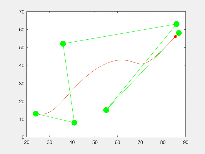
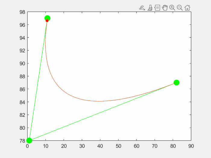
这是用彗星图画的
P=randi(100,2,60);
position=computeCubicBezierCurve(P,100);

X=position(1,:);
Y=position(2,:);
figure(1);
h=gca;
plot(P(1,:),P(2,:),'g.-','MarkerSize',40);
c={
   '起点'};
text(P(1,1),P(2,1),c,'HorizontalAlignment','left')
hold on

text(P(1,end),P(2,end),'终点','HorizontalAlignment','left')
hold on

mycomet(h,X,Y,0.8)
2.1总代码
clc;clear;
% fps = 40;
% myVideo = VideoWriter('test2.avi');
% myVideo.FrameRate = fps;
% open(myVideo);
% P0=[1,2];
% P1=[5,8];
% P2=[10,10];
% P=[P0;P1;P2];
% X=@(t)(1-t).^2.*P0(1)+2.*t.*(1-t)*P1(1)+t.^2*P2(1);
% Y=@(t)(1-t).^2.*P0(2)+2.*t.*(1-t)*P1(2)+t.^2*P2(2);
% x1=@(t)(1-t).*P0(1)+t.*P1(1);
% y1=@(t)(1-t).*P0(2)+t.*P1(2);
% x2=@(t)(1-t).*P1(1)+t.*P2(1);
% y2=@(t)(1-t).*P1(2)+t.*P2(2);
% t=0:0.01:1;
% X=X(t);
% Y=Y(t);
% x1=x1(t);
% y1=y1(t);
% x2=x2(t);
% y2=y2(t);
P=randi(100,2,6);
position=computeCubicBezierCurve(P,100);

X=position(1,:);
Y=position(2,:);
% figure(1);
% h=gca;
% plot(P(1,:),P(2,:),'g.-','MarkerSize',40);
% c={'起点'};
% text(P(1,1),P(2,1),c,'HorizontalAlignment','left')
% hold on
%
% text(P(1,end),P(2,end),'终点','HorizontalAlignment','left')
% hold on
%
% mycomet(h,X,Y,0.8)

% figure
% for k = 1:101
%     plot(P(1,:),P(2,:),'k.-','MarkerSize',40),hold on
%     plot(X(k),Y(k),'r.'),hold on
%     % plot(x1(k),y1(k),'g.'),hold on
%     % plot(x2(k),y2(k),'g.'),hold on
%     % plot([x2(k),x1(k)],[y2(k),y1(k)],'y-'),hold on
%     axis([min(P(1,:)),max(P(1,:)),min(P(2,:)),max(P(2,:))]),drawnow
%     frame = getframe(gcf);
%     im = frame2im(frame);
%     writeVideo(myVideo,im);
% end
% close(myVideo);
plot(P(1,:),P(2,:),'g.-','MarkerSize',40),hold on
plot(X,Y)
hold on
p = plot(X(1),Y(1),'o','MarkerFaceColor','red');
hold off
axis manual
pic_num=1;
for k = 2:101
    p.XData = X(k);
    p.YData = Y(k);

    F=getframe(gcf);
    I=frame2im(F);
    [I,map]=rgb2ind(I,256);
    if pic_num==1
    imwrite(I,map,'test.gif','gif','Loopcount',inf,'DelayTime',0.2);
    elseif mod(pic_num,3)==1
    imwrite(I,map,'test.gif','gif','WriteMode','append','DelayTime',0.2);
    end
    pic_num = pic_num + 1;

    drawnow limitrate
end
function mycomet(varargin)
%COMET  Comet-like trajectory.
%   COMET(Y) displays an animated comet plot of the vector Y.
%   COMET(X,Y) displays an animated comet plot of vector Y vs. X.
%   COMET(X,Y,p) uses a comet of length p*length(Y).  Default is p = 0.10.
%
%   COMET(AX,...) plots into AX instead of GCA.
%
%   Example:
%       t = -pi:pi/200:pi;
%       comet(t,tan(sin(t))-sin(tan(t)))
%
%   See also COMET3.

%   Charles R. Denham, MathWorks, 1989.
%   Copyright 1984-2022 The MathWorks, Inc.

% Parse possible Axes input
nnn=0.05;

[ax,args,nargs] = axescheck(varargin{
   :});
if nargs < 1
    error(message('MATLAB:narginchk:notEnoughInputs'));
elseif nargs > 3
    error(message('MATLAB:narginchk:tooManyInputs'));
end

% Parse the rest of the inputs
bodyLengthProportion = 0.10;
if nargs < 2, x = args{
   1}; y = x; x = 1:length(y); end
if nargs == 2, [x,y] = deal(args{
   :}); end
if nargs == 3, [x,y,bodyLengthProportion] = deal(args{
   :}); end

if ~isscalar(bodyLengthProportion) || ~isreal(bodyLengthProportion) ||  bodyLengthProportion < 0 || bodyLengthProportion >= 1
    error(message('MATLAB:comet:InvalidP'));
end

x = matlab.graphics.chart.internal.datachk(x);
y = matlab.graphics.chart.internal.datachk(y);

if ~isvector(x) || ~isvector(y) || numel(x) ~= numel(y)
    error(message('MATLAB:comet:XYVectorsSameLength'));
end

ax = newplot(ax);

if ~strcmp(ax.NextPlot,'add')
    % If NextPlot is 'add', assume other objects are driving the limits.
    % Otherwise, set the limits so that the axes limits don't jump around
    % during animation.
    [minx,maxx] = minmax(x);
    [miny,maxy] = minmax(y);
    if ~isa(ax,'matlab.graphics.axis.GeographicAxes') && ~isa(ax,'map.graphics.axis.MapAxes')
        axis(ax,[minx maxx miny maxy])
    else
        % Latitudes are the first axis (x) and longitudes are the second
        % axis (y).
        latmin = minx;
        latmax = maxx;
        lonmin = miny;
        lonmax = maxy;

        % Buffer the limits for better display.
        bufferInPercent = 5;
        f = 1 + bufferInPercent / 100;
        half = f * (latmax - latmin)/2;
        latlim = [-half, half] + (latmin + latmax)/2;
        latlim(1) = max(latlim(1), -90);
        latlim(2) = min(latlim(2),  90);
        half = f * (lonmax - lonmin)/2;
        lonlim = [-half, half] + (lonmin + lonmax)/2;

        geolimits(ax,latlim,lonlim)
    end
end

totalLength = length(x);
bodyLength = round(bodyLengthProportion*totalLength);

head = line('Parent',ax,'SeriesIndex_I',0,'Marker','o','LineStyle','none', ...
            'XData',x(1),'YData',y(1),'Tag','head');
body = matlab.graphics.animation.AnimatedLine('SeriesIndex_I',0,...
    'Parent',ax,'MaximumNumPoints',max(1,bodyLength),'tag','body');
tail = matlab.graphics.animation.AnimatedLine('Parent',ax, 'SeriesIndex_I',0,...
    'LineStyle','-','MaximumNumPoints',1+totalLength,'tag','tail'); %Add 1 for any extra points

if isequal(body.Color,tail.Color) && isequal(body.LineStyle, tail.LineStyle)
    body.LineStyle='--';
end

if length(x) < 2000
    updateFcn = @()drawnow;
else
    updateFcn = @()drawnow('limitrate');
end

% Grow the body
for i = 1:bodyLength
    % Protect against deleted objects following the call to drawnow.
    if ~(isvalid(head) && isvalid(body))
        return
    end
    set(head,'xdata',x(i),'ydata',y(i));
    addpoints(body,x(i),y(i));
    updateFcn();
    pause(nnn)
end

% Add a drawnow to capture any events / callbacks
drawnow

% Initialize tail with first point. The next point will be added in the
% first iteration of the primary loop below, creating the first line
% segment of the tail.
addpoints(tail,x(1),y(1));

% Primary loop
for i = bodyLength+1:totalLength
    % Protect against deleted objects following the call to drawnow.
    if ~(isvalid(head) && isvalid(body) && isvalid(tail))
        return
    end
    set(head,'xdata',x(i),'ydata',y(i));
    addpoints(body,x(i),y(i));

    nextTailIndex = i-bodyLength+1;
    if(nextTailIndex<=totalLength)
        addpoints(tail,x(nextTailIndex),y(nextTailIndex));
    end
    updateFcn();
    pause(nnn)
end
drawnow

% Allow tail to continue on to the full length. The last point added to the
% tail in the primary loop above was at index (totalLength-bodyLength+1),
% so this loop starts at the following index.
for i = totalLength-bodyLength+2:totalLength
    % Protect against deleted objects following the call to drawnow.
    if ~isvalid(tail)
        return
    end
    addpoints(tail,x(i),y(i));
    updateFcn();
    pause(nnn)
end
drawnow

end

function [minx,maxx] = minmax(x)
minx = min(x(isfinite(x)));
maxx = max(x(isfinite(x)));
if minx == maxx
    minx = maxx-1;
    maxx = maxx+1;
end
end
function points = computeCubicBezierCurve(controlPoints, numPoints)
    numControlPoints = size(controlPoints, 2);
    t = linspace(0, 1, numPoints); % 在0到1之间生成numPoints个等间距的参数值
    points = zeros(2, numPoints); % 存储曲线上的点坐标

    for i = 1:numPoints
        B = zeros(2, 1);
        for j = 1:numControlPoints
            B = B + nchoosek(numControlPoints-1, j-1) * t(i)^(j-1) * (1 - t(i))^(numControlPoints-j) * controlPoints(:, j);
        end
        points(:, i) = B; % 存储点坐标
    end
end
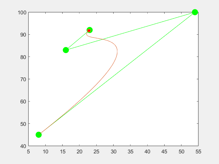
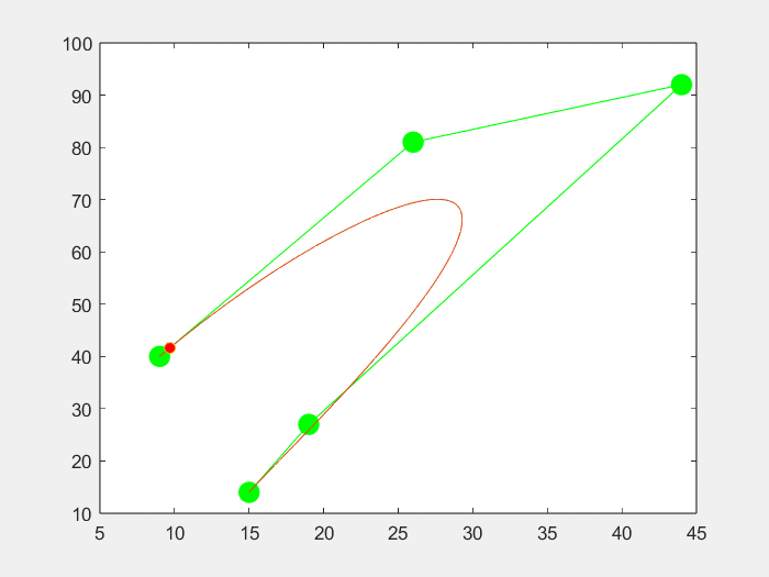
3.效果
三个点
四个点
五个点
六个点