1. Introduction
We are drowning in data, but starving for knowledge. (John Naisbitt, 1982)
Data mining draws ideas from machine learning, statistics, and database systems.
Methods
| Descriptive methods = unsupervised | Predictive methods = supervised |
|---|---|
| with a target (class) attribute | no target attribute |
| Clustering, Association Rule Mining, Text Mining, Anomaly Detection, Sequential Pattern Mining | Classification, Regression, Text Mining, Time Series Prediction |
None of the data mining steps actually require a computer. But computers are scalability and they can help avoid human bias.
Basic process:
Apply data mining method -> Evaluate resulting model / patterns -> Iterate:
– Experiment with different parameter settings
– Experiment with different alternative methods
– Improve preprocessing and feature generation
– Combine different methods
2. Clustering
Intra-cluster distances are minimized: Data points in one cluster are similar to one another.
Inter-cluster distances are maximized: Data points in separate clusters are different from each other.
Application area: Market segmentation, Document Clustering
Types:
- Partitional Clustering: A division data objects into non-overlapping subsets (clusters) such that each data object is in exactly one subset
- Hierarchical Clustering: A set of nested clusters organized as a hierarchical tree
**Clustering algorithm: ** Partitional, Hierarchical, Density-based Algorithms
**Proximity (similarity, or dissimilarity) measure: ** Euclidean Distance, Cosine Similarity, Domain-specific Similarity Measures
Application area: Product Grouping, Social Network Analysis, Grouping Search Engine Results, Image Recognition
2.1 K-Means Clustering
- partitional clustering
- each cluster is associated with a centroid
- each point is assigned to the cluster with the closest centroid
- number of clusters must be specified manually

- Convergence Criteria
- no (or minimum) re-assignments of data points to different clusters
- no (or minimum) change of centroids,
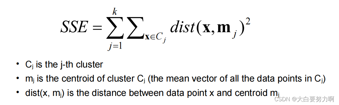
- minimum decrease in the sum of squared errors (SSE)
- Stop after X iterations
Weaknesses1: Initial Seeds
Results can vary significantly depending on the initial choice of seeds (number and position)
Improving:
- Restart a number of times with different random seeds (but fixed k)
- Run k-means with different values of k -> Choose k where SSE improvement decreases (knee value of k)
- Employ X-Means: variation of K-Means algorithm that automatically determines k. Starts with a small k, then splits large clusters until improvement decreases.
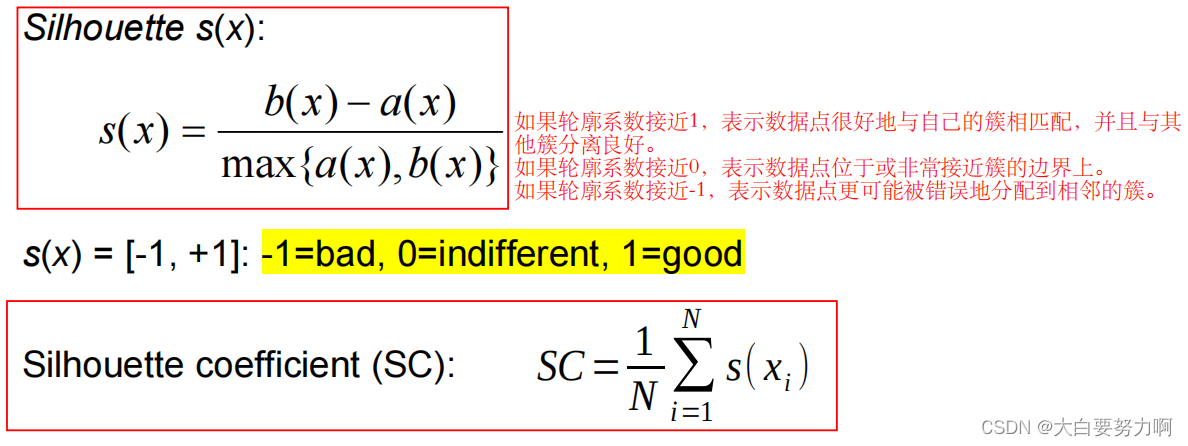
- Run k-means with different k values and Plot the Silhouette Coefficient -> Pick the best (i.e., highest) silhouette coefficient
Weaknesses2: Outlier Handling
Remedy:
- remove data points far away from centroids
- random sampling
Choose a small subset of the data points. The chance of selecting an outlier is very small if the data set is large enough. After determining the centroids based on samples, assign the rest of the data points. It’s also a method for improving runtime performance!
Evaluation
maximize Cohesion & Separation
- Cohesion a(x): average distance of x to all other vectors in the same cluster. 是数据点x到同一簇中其他点的平均距离(簇内平均距离)。
- Separation b(x): average distance of x to the vectors in other clusters. Find the minimum among the clusters.数据点x到最近的相邻簇中所有点的平均距离(与最近簇的平均距离)。
Silhouette coefficient
The silhouette coefficient does not depend on the number of clusters.
summary
Advantages: Simple, Efficient time complexity: O(tkn) [n: number of data points, k: number of clusters, t: number of iterations]
Disadvantages: Must pick number of clusters before hand; All items are forced into a
cluster; Sensitive to outliers; Sensitve to initial seeds
2.2 K-Medoids
K-Medoids is a K-Means variation that uses the medians of each cluster instead of the mean.
Medoids are the most central existing data points in each cluster
K-Medoids is more robust against outliers as the median is not affected by extreme values
2.3 DBSCAN
DBSCAN: Density-Based Spatial Clustering of Applications with Noise
density-based algorithm
Density = number of points within a specified radius (Eps)
- core point: it has more than a specified number of points (MinPts) within Eps, including the point itself
- border point: it has fewer than MinPts within Eps, but is in the neighborhood of a core point
- noise point: any point that is not a core point or a border point
DBSCAN Algorithm: Eliminate noise points -> Perform clustering on the remaining points
Advantages: Resistant to Noise + Can handle clusters of different shapes and sizes
Disadvantages: Varying densities + High-dimensional data
Determining EPS and MinPts?
- For points in a cluster, their kth nearest neighbors are at roughly the same distance对于一个簇中的点,它们的第k个最近邻大致在相同的距离。这意味着在一个簇内,数据点的第 k 个最近邻应该大致位于相同的距离范围内。这是因为在一个簇中的点应该彼此靠近。
- Noise points have the kth nearest neighbor at farther distance. 噪声点的第k个最近邻在更远的距离。对于噪声点,它们的第 k 个最近邻应该位于相对较远的距离。这是因为噪声点通常是离群值,与其他点相对较远。
- Plot sorted distance of every point to its kth nearest neighbor. 在 k-distance plot 中,拐点是指图上出现的一个明显的拐角或拐点,也就是距离开始增长更快的位置。这个拐点通常对应于数据中的一个自然分界点,标志着在这个点之后,点与其 kth 最近邻的距离开始显著增加。这个点的选择通常作为确定 EPS(邻域半径)的参考值。在 k-distance plot 中,横轴表示数据点到其第 k 个最近邻的距离,纵轴表示这些距离的排序。拐点处的距离通常可以作为一个合适的 EPS 值,因为这个点之后的距离增长较快,表明这个位置可能是簇的边界。
2.4 Hierarchical Clustering
Produces a set of nested clusters organized as a hierarchical tree. Can be visualized as a Dendrogram. (A tree like diagram that records the sequences of merges or splits. The y-axis displays the former distance between merged clusters.)
Advantages: We do not have to assume any particular number of clusters. May be used to look for meaningful taxonomies.
Step:
Starting Situation: Start with clusters of individual points and a proximity matrix
Intermediate Situation: After some merging steps, we have a number of clusters.
How to Define Inter-Cluster Similarity?
- Single Link (MIN): Similarity of two clusters is based on the two most similar (closest) points in the different clusters. 求解最近距离之间的最小值. Can handle non-elliptic shapes but Sensitive to outliers.
- Complete Link (MAX): Similarity of two clusters is based on the two least similar (most distant) points in the different clusters. 求解最远距离之间的最小值。Less sensitive to noise and outliers but biased towards globular clusters and tends to break large clusters.
- Group Average: average of pair-wise
proximity between points in the two clusters. Need to use average connectivity for scalability since total proximity favors large clusters. Compromise between Single and Complete Link. Less susceptible to noise and outliers but Biased towards globular clusters - Distance Between Centroids
Limitations
- Greedy algorithm: decision taken cannot be undone
- Different variants have problems with one or more of the following: Sensitivity to noise and outliers, Difficulty handling different sized clusters and convex shapes, Breaking large clusters
- High Space and Time Complexity[O(N^2
) space, O(N^3) time]
2.5 Proximity Measures
Single Attributes: Similarity [0,1] and Dissimilarity [0, upper limit varies]
Many Mttributes:
Euclidean Distance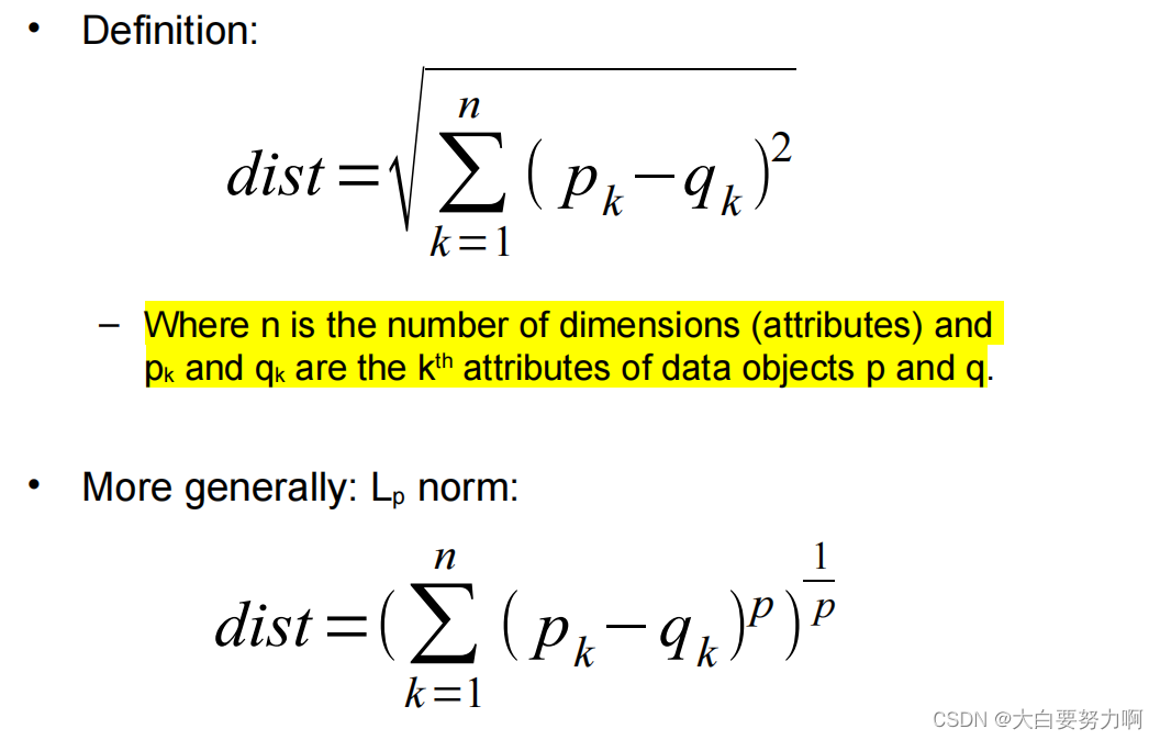
Caution
We are easily comparing apples and oranges.
changing units of measurement -> changes the clustering result
Recommendation: use normalization before clustering(generally, for all data mining algorithms involving distances)
Similarity of Binary Attributes
Common situation is that objects, p and q, have only binary attributes
1.Symmetric Binary Attributes -> hobbies, favorite bands, favorite movies
A binary attribute is symmetric if both of its states (0 and 1) have
equal importance, and carry the same weights
Similarity measure: Simple Matching Coefficient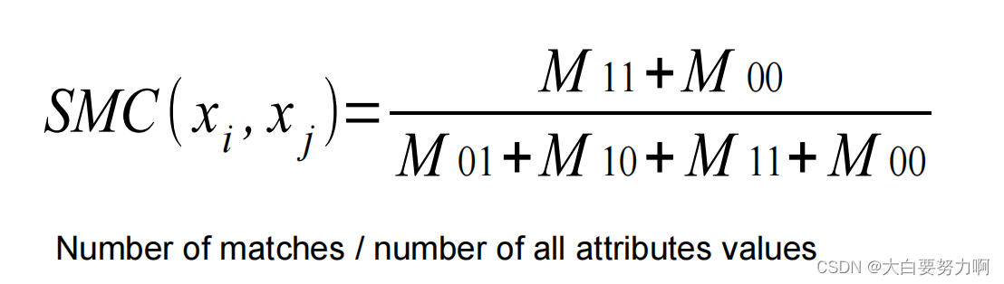
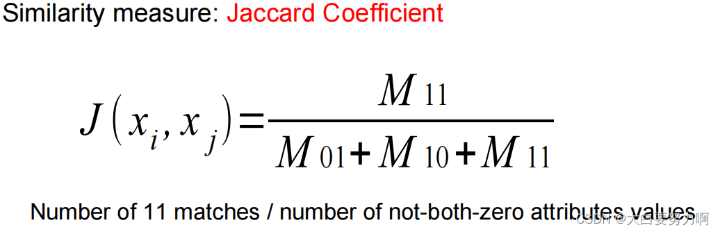
2.Asymmetric Binary Attributes -> (dis-)agreement with political statements, recommendation for voting
Asymmetric: If one of the states is more important or more valuable than the other. By convention, state 1 represents the more important state. 1 is typically the rare or infrequent state. Example: Shopping Basket, Word/Document Vector
Association Rule Discovery
Given a set of records each of which contains some number of items from a given collection.
Produce dependency rules that will predict the occurrence of an item based on occurrences of other items.
Application area: Marketing and Sales Promotion, Content-based recommendation, Customer loyalty programs