本文为李沐老师《动手学深度学习》笔记小结,用于个人复习并记录学习历程,适用于初学者
神经网络架构设计的模块化
然AlexNet证明深层神经网络卓有成效,但它没有提供一个通用的模板来指导后续的研究人员设计新的网络。 在下面的几个章节中,我们将介绍一些常用于设计深层神经网络的启发式概念。
与芯片设计中工程师从放置晶体管到逻辑元件再到逻辑块的过程类似,神经网络架构的设计也逐渐变得更加抽象。研究人员开始从单个神经元的角度思考问题,发展到整个层,现在又转向块,重复层的模式。
使用块的想法首先出现在牛津大学的视觉几何组(visual geometry group)的VGG网络中。通过使用循环和子程序,可以很容易地在任何现代深度学习框架的代码中实现这些重复的架构。
VGG架构
VGG块
经典卷积神经网络的基本组成部分是下面的这个序列:
- 带填充以保持分辨率的卷积层;
- 非线性激活函数,如ReLU;
- 汇聚层,如最大汇聚层。
而一个VGG块与之类似,由一系列卷积层组成,后面再加上用于空间下采样的最大汇聚层。在最初的VGG论文中 ,作者了带有3×3卷积核、填充为1(保持高度和宽度)的卷积层,和带有2×2汇聚窗口、步幅为2(每个块后的分辨率减半)的最大汇聚层。
import torch
from torch import nn

def vgg_block(num_convs, in_channels, out_channels):
    layers = []
    for _ in range(num_convs):
        layers.append(nn.Conv2d(in_channels, out_channels,
                                kernel_size=3, padding=1))
        layers.append(nn.ReLU())
        in_channels = out_channels
    layers.append(nn.MaxPool2d(kernel_size=2,stride=2))
    return nn.Sequential(*layers)
VGG网络
与AlexNet、LeNet一样,VGG网络可以分为两部分:第一部分主要由卷积层和汇聚层组成,第二部分由全连接层组成。
原始VGG网络有5个卷积块,其中前两个块各有一个卷积层,后三个块各包含两个卷积层。 第一个模块有64个输出通道,每个后续模块将输出通道数量翻倍,直到该数字达到512。由于该网络使用8个卷积层和3个全连接层,因此它通常被称为VGG-11。

这里我们构建比书上还要小的网络用于训练。
def vgg(conv_arch):
    conv_blks = []
    in_channels = 1
    # 卷积层部分
    for (num_convs, out_channels) in conv_arch:
        conv_blks.append(vgg_block(num_convs, in_channels, out_channels))
        in_channels = out_channels

    return nn.Sequential(
        *conv_blks, nn.Flatten(),
        # 全连接层部分
        nn.Linear(out_channels * 5 * 5, 1024), nn.ReLU(), nn.Dropout(0.5),
        nn.Linear(1024, 128), nn.ReLU(), nn.Dropout(0.5),
        nn.Linear(128, 10))

conv_arch = ((1, 64), (1, 128), (2, 256), (2, 512), (2, 512)) #这里(2,256)2指重复两次
net = vgg(conv_arch)接下来,我们将构建一个高度和宽度为160的单通道数据样本,以[观察每个层输出的形状]。
X = torch.randn(size=(1, 1, 160, 160))
for blk in net:
    X = blk(X)
    print(blk.__class__.__name__,'output shape:\t',X.shape)
输出:
Sequential output shape:	 torch.Size([1, 64, 80, 80])
Sequential output shape:	 torch.Size([1, 128, 40, 40])
Sequential output shape:	 torch.Size([1, 256, 20, 20])
Sequential output shape:	 torch.Size([1, 512, 10, 10])
Sequential output shape:	 torch.Size([1, 512, 5, 5])
Flatten output shape:	 torch.Size([1, 12800])
Linear output shape:	 torch.Size([1, 1024])
ReLU output shape:	 torch.Size([1, 1024])
Dropout output shape:	 torch.Size([1, 1024])
Linear output shape:	 torch.Size([1, 128])
ReLU output shape:	 torch.Size([1, 128])
Dropout output shape:	 torch.Size([1, 128])
Linear output shape:	 torch.Size([1, 10])
训练模型
缩小模型
拿Fashion-MNIST数据集,我们可以再次减小通道数。
ratio = 4
small_conv_arch = [(pair[0], pair[1] // ratio) for pair in conv_arch]
net = vgg(small_conv_arch)

X = torch.randn(size=(1, 1, 160, 160))
for blk in net:
    X = blk(X)
    print(blk.__class__.__name__,'output shape:\t',X.shape)
输出:
Sequential output shape:	 torch.Size([1, 16, 80, 80])
Sequential output shape:	 torch.Size([1, 32, 40, 40])
Sequential output shape:	 torch.Size([1, 64, 20, 20])
Sequential output shape:	 torch.Size([1, 128, 10, 10])
Sequential output shape:	 torch.Size([1, 128, 5, 5])
Flatten output shape:	 torch.Size([1, 3200])
Linear output shape:	 torch.Size([1, 1024])
ReLU output shape:	 torch.Size([1, 1024])
Dropout output shape:	 torch.Size([1, 1024])
Linear output shape:	 torch.Size([1, 128])
ReLU output shape:	 torch.Size([1, 128])
Dropout output shape:	 torch.Size([1, 128])
Linear output shape:	 torch.Size([1, 10])
预备工作
from IPython import display
import torchvision
from torch.utils import data
from torchvision import transforms
import matplotlib.pyplot as plt

def load_data_fashion_mnist(batch_size, resize=None):
    """下载Fashion-MNIST数据集,然后将其加载到内存中"""
    trans = [transforms.ToTensor()]
    if resize:
        trans.insert(0, transforms.Resize(resize))
    trans = transforms.Compose(trans)
    mnist_train = torchvision.datasets.FashionMNIST(
        root="../data", train=True, transform=trans, download=0)
    mnist_test = torchvision.datasets.FashionMNIST(
        root="../data", train=False, transform=trans, download=0)
    return (data.DataLoader(mnist_train, batch_size, shuffle=True,
                            num_workers=get_dataloader_workers()),
            data.DataLoader(mnist_test, batch_size, shuffle=False,
                            num_workers=get_dataloader_workers()))

def get_dataloader_workers():
    """使用4个进程来读取数据"""
    return 4

batch_size = 128
train_iter, test_iter = load_data_fashion_mnist(batch_size, resize=160)

def accuracy(y_hat, y):  #@save
    """计算预测正确的数量"""
    if len(y_hat.shape) > 1 and y_hat.shape[1] > 1:
        y_hat = y_hat.argmax(axis=1) #找出输入张量(tensor)中最大值的索引
    cmp = y_hat.type(y.dtype) == y
    return float(cmp.type(y.dtype).sum())
class Accumulator:  #@save
    """在n个变量上累加"""
    def __init__(self, n):
        self.data = [0.0] * n

    def add(self, *args):
        self.data = [a + float(b) for a, b in zip(self.data, args)]

    def reset(self):
        self.data = [0.0] * len(self.data)

    def __getitem__(self, idx):
        return self.data[idx]

import matplotlib.pyplot as plt
from matplotlib_inline import backend_inline

def use_svg_display():
    """使⽤svg格式在Jupyter中显⽰绘图"""
    backend_inline.set_matplotlib_formats('svg')

def set_axes(axes, xlabel, ylabel, xlim, ylim, xscale, yscale, legend):
     """设置matplotlib的轴"""
     axes.set_xlabel(xlabel)
     axes.set_ylabel(ylabel)
     axes.set_xscale(xscale)
     axes.set_yscale(yscale)
     axes.set_xlim(xlim)
     axes.set_ylim(ylim)
     if legend:
         axes.legend(legend)
     axes.grid()

class Animator:  #@save
    """在动画中绘制数据"""
    def __init__(self, xlabel=None, ylabel=None, legend=None, xlim=None,
                 ylim=None, xscale='linear', yscale='linear',
                 fmts=('-', 'm--', 'g-.', 'r:'), nrows=1, ncols=1,
                 figsize=(3.5, 2.5)):
        # 增量地绘制多条线
        if legend is None:
            legend = []
        use_svg_display()
        self.fig, self.axes = plt.subplots(nrows, ncols, figsize=figsize)
        if nrows * ncols == 1:
            self.axes = [self.axes, ]
        # 使用lambda函数捕获参数
        self.config_axes = lambda: set_axes(
            self.axes[0], xlabel, ylabel, xlim, ylim, xscale, yscale, legend)
        self.X, self.Y, self.fmts = None, None, fmts

    def add(self, x, y):
        # 向图表中添加多个数据点
        if not hasattr(y, "__len__"):
            y = [y]
        n = len(y)
        if not hasattr(x, "__len__"):
            x = [x] * n
        if not self.X:
            self.X = [[] for _ in range(n)]
        if not self.Y:
            self.Y = [[] for _ in range(n)]
        for i, (a, b) in enumerate(zip(x, y)):
            if a is not None and b is not None:
                self.X[i].append(a)
                self.Y[i].append(b)
        self.axes[0].cla()
        for x, y, fmt in zip(self.X, self.Y, self.fmts):
            self.axes[0].plot(x, y, fmt)
        self.config_axes()
        display.display(self.fig)
        display.clear_output(wait=True)

def evaluate_accuracy_gpu(net, data_iter, device=None): #@save
    """使用GPU计算模型在数据集上的精度"""
    if isinstance(net, nn.Module):
        net.eval()  # 设置为评估模式
        if not device:
            device = next(iter(net.parameters())).device
    # 正确预测的数量,总预测的数量
    metric = Accumulator(2)
    with torch.no_grad():
        for X, y in data_iter:
            if isinstance(X, list):
                # BERT微调所需的(之后将介绍)
                X = [x.to(device) for x in X]
            else:
                X = X.to(device)
            y = y.to(device)
            metric.add(accuracy(net(X), y), y.numel())
    return metric[0] / metric[1]

import time
class Timer:  #@save
    """记录多次运行时间"""
    def __init__(self):
        self.times = []
        self.start()

    def start(self):
        """启动计时器"""
        self.tik = time.time()

    def stop(self):
        """停止计时器并将时间记录在列表中"""
        self.times.append(time.time() - self.tik)
        return self.times[-1]

    def avg(self):
        """返回平均时间"""
        return sum(self.times) / len(self.times)

    def sum(self):
        """返回时间总和"""
        return sum(self.times)

    def cumsum(self):
        """返回累计时间"""
        return np.array(self.times).cumsum().tolist()

def train_ch6(net, train_iter, test_iter, num_epochs, lr, device):
    """用GPU训练模型(在第六章定义)"""
    def init_weights(m):
        if type(m) == nn.Linear or type(m) == nn.Conv2d:
            nn.init.xavier_uniform_(m.weight)
    net.apply(init_weights)
    print('training on', device)
    net.to(device)
    optimizer = torch.optim.SGD(net.parameters(), lr=lr)
    loss = nn.CrossEntropyLoss()
    animator = Animator(xlabel='epoch', xlim=[1, num_epochs],
                            legend=['train loss', 'train acc', 'test acc'])
    timer, num_batches = Timer(), len(train_iter)
    for epoch in range(num_epochs):
        # 训练损失之和,训练准确率之和,样本数
        metric = Accumulator(3)
        net.train()
        for i, (X, y) in enumerate(train_iter):
            timer.start()
            optimizer.zero_grad()
            X, y = X.to(device), y.to(device)
            y_hat = net(X)
            l = loss(y_hat, y)
            l.backward()
            optimizer.step()
            with torch.no_grad():
                metric.add(l * X.shape[0], accuracy(y_hat, y), X.shape[0])
            timer.stop()
            train_l = metric[0] / metric[2]
            train_acc = metric[1] / metric[2]
            if (i + 1) % (num_batches // 5) == 0 or i == num_batches - 1:
                animator.add(epoch + (i + 1) / num_batches,
                             (train_l, train_acc, None))
        test_acc = evaluate_accuracy_gpu(net, test_iter)
        animator.add(epoch + 1, (None, None, test_acc))
    print(f'loss {train_l:.3f}, train acc {train_acc:.3f}, '
          f'test acc {test_acc:.3f}')
    print(f'{metric[2] * num_epochs / timer.sum():.1f} examples/sec '
          f'on {str(device)}')

def try_gpu(i=0):  #@save
    """如果存在,则返回gpu(i),否则返回cpu()"""
    if torch.cuda.device_count() >= i + 1:
        return torch.device(f'cuda:{i}')
    return torch.device('cpu')
模型训练
lr, num_epochs, batch_size = 0.05, 10, 128
train_iter, test_iter = load_data_fashion_mnist(batch_size, resize=160)
begin = time.time()
train_ch6(net, train_iter, test_iter, num_epochs, lr, try_gpu())
end = time.time()
print(end - begin)
这个结果可以说相当不错,对比我完全没调整参数的AlexNet,不仅训练速度更快,并且效果更好。
 小结
小结
- VGG-11使用可复用的卷积块构造网络。不同的VGG模型可通过每个块中卷积层数量和输出通道数量的差异来定义。
- 块的使用导致网络定义的非常简洁。使用块可以有效地设计复杂的网络。
- 在VGG论文中,Simonyan和Ziserman尝试了各种架构。特别是他们发现深层且窄的卷积(即3×3)比较浅层且宽的卷积更有效。