1. 发展历史
遗传算法(Genetic Algorithm, GA)是一种受自然选择和遗传学启发的优化算法。它最早由美国学者John Holland在20世纪70年代提出,旨在研究自然系统中的适应性,并应用于计算机科学中的优化问题。
关键发展历程
1975年: John Holland在其著作《Adaptation in Natural and Artificial Systems》中首次提出遗传算法的概念。
1980年代: 遗传算法开始应用于函数优化、组合优化等领域,逐渐受到关注。
1990年代: 随着计算机计算能力的提升,遗传算法在工程、经济学、生物学等领域得到广泛应用。
2000年代至今: 遗传算法的理论和应用进一步发展,出现了多种改进算法,如
遗传编程(Genetic Programming)、差分进化(Differential Evolution)等。
2. 数学原理
遗传算法是一种基于自然选择和遗传学的随机搜索方法,其基本思想是模拟生物进化过程,通过选择、交叉和变异操作,不断产生新一代种群,从而逐步逼近最优解。
遗传算法的基本步骤
初始化: 随机生成初始种群。
选择: 根据适应度函数选择较优个体。
交叉: 通过交换父代个体的部分基因产生新个体。
变异: 随机改变个体的部分基因。
迭代: 重复选择、交叉、变异过程,直到满足终止条件。
数学描述
假设种群大小为N,每个个体的染色体长度为L,遗传算法的数学过程如下:
初始化: 生成种群 ,其中 为染色体。
适应度计算: 计算每个个体的适应度值 。
选择: 根据适应度值选择个体,常用方法有轮盘赌选择、锦标赛选择等。
交叉: 选取部分个体进行交叉操作,产生新个体 。
变异: 对部分新个体进行变异操作,产生变异个体 。
更新种群: 用新个体替换旧个体,形成新一代种群 。
终止条件: 若达到预设的终止条件(如迭代次数或适应度阈值),则输出最优解。
3. 应用场景
遗传算法因其适应性和鲁棒性,在多种领域得到了广泛应用:
工程优化
结构优化: 设计轻量化和高强度的结构。
参数优化: 调整系统参数以达到最佳性能。
经济学与金融
投资组合优化: 分配投资资产以最大化收益。
市场预测: 预测股票价格和市场趋势。
生物信息学
基因序列比对: 进行DNA序列的比对和分析。
蛋白质结构预测: 预测蛋白质的三维结构。
机器学习
神经网络训练: 优化神经网络的权重和结构。
特征选择: 选择最有利于分类或回归的特征。
4. 可视化实现Python实例
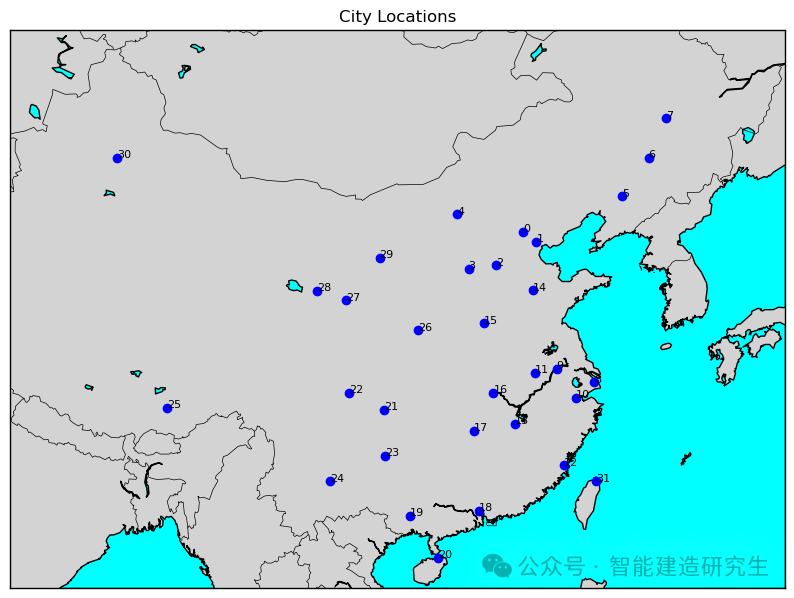
以下代码示例实现了一个解决旅行商问题的遗传算法。旅行商问题(TSP)是一个经典的组合优化问题,旨在找到一个旅行商从一组给定城市中的每一个城市恰好访问一次,并最终回到起始城市的最短路径,即最小化总旅行距离或成本,广泛应用于物流、生产调度等领域。
我们首先定义中国所有省会城市(包含中国台湾省省会台北)及其坐标的数据,并使用哈夫曼公式计算两点间的距离,然后通过遗传算法创建初始种群,进行繁殖、突变和生成下一代,不断优化路径,最终记录每一代中最短路径的距离和对应的路径,并在所有迭代中找到最短路径,在地图上可视化展示所有城市位置、适应度随迭代次数变化以及最优路径,最终结果展示了从重庆出发经过所有城市的最短路径及其总距离。总共训练两次,第一次迭代次数为2000次,运行时间约为3分钟,第二次设置迭代次数20000次,运行时间大概在15分钟左右。
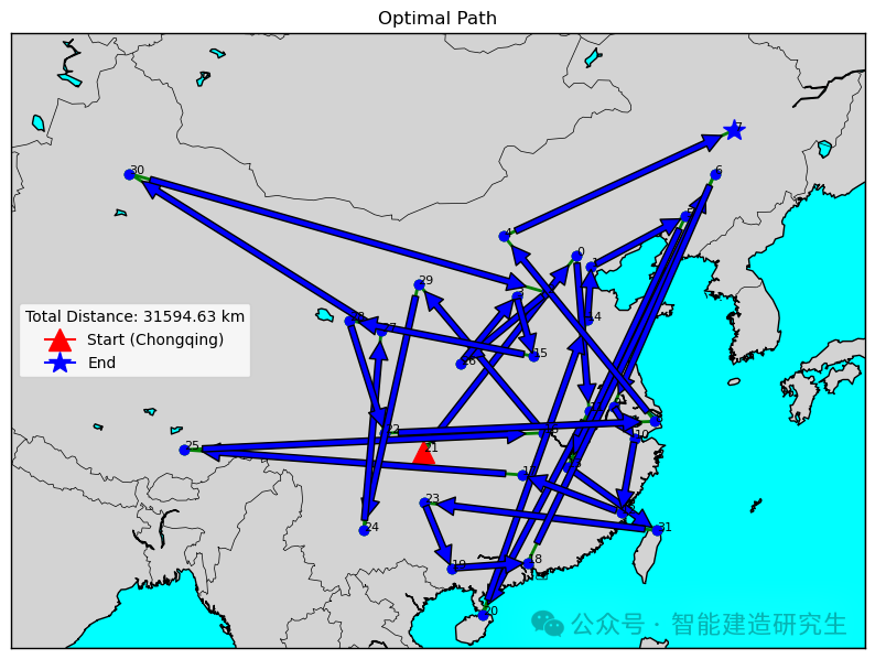
用一句话总结:从重庆出发,游遍中国所有的省会城市,利用遗传算法寻找到最短路径。以下是代码实现:
import numpy as np
import matplotlib.pyplot as plt
from mpl_toolkits.basemap import Basemap
import random
from math import radians, sin, cos, sqrt, atan2
# 设置随机种子以保证结果可重复
random.seed(42)
np.random.seed(42)
# 定义城市和坐标列表,包括台北
cities = {
"北京": (39.9042, 116.4074),
"天津": (39.3434, 117.3616),
"石家庄": (38.0428, 114.5149),
"太原": (37.8706, 112.5489),
"呼和浩特": (40.8426, 111.7511),
"沈阳": (41.8057, 123.4315),
"长春": (43.8171, 125.3235),
"哈尔滨": (45.8038, 126.5349),
"上海": (31.2304, 121.4737),
"南京": (32.0603, 118.7969),
"杭州": (30.2741, 120.1551),
"合肥": (31.8206, 117.2272),
"福州": (26.0745, 119.2965),
"南昌": (28.6820, 115.8579),
"济南": (36.6512, 117.1201),
"郑州": (34.7466, 113.6254),
"武汉": (30.5928, 114.3055),
"长沙": (28.2282, 112.9388),
"广州": (23.1291, 113.2644),
"南宁": (22.8170, 108.3665),
"海口": (20.0174, 110.3492),
"重庆": (29.5638, 106.5507),
"成都": (30.5728, 104.0668),
"贵阳": (26.6477, 106.6302),
"昆明": (25.0460, 102.7097),
"拉萨": (29.6520, 91.1721),
"西安": (34.3416, 108.9398),
"兰州": (36.0611, 103.8343),
"西宁": (36.6171, 101.7782),
"银川": (38.4872, 106.2309),
"乌鲁木齐": (43.8256, 87.6168),
"台北": (25.032969, 121.565418)
}
# 城市列表和坐标
city_names = list(cities.keys())
locations = np.array(list(cities.values()))
chongqing_index = city_names.index("重庆")
# 使用哈夫曼公式计算两点间的距离
def haversine(lat1, lon1, lat2, lon2):
R = 6371.0 # 地球半径,单位为公里
dlat = radians(lat2 - lat1)
dlon = radians(lon1 - lon2)
a = sin(dlat / 2)**2 + cos(radians(lat1)) * cos(radians(lat2)) * sin(dlon / 2)**2
c = 2 * atan2(sqrt(a), sqrt(1 - a))
distance = R * c
return distance
# 计算路径总距离的函数,单位为公里
def calculate_distance(path):
return sum(haversine(locations[path[i]][0], locations[path[i]][1], locations[path[i + 1]][0], locations[path[i + 1]][1]) for i in range(len(path) - 1))
# 创建初始种群
def create_initial_population(size, num_cities):
population = []
for _ in range(size):
individual = random.sample(range(num_cities), num_cities)
# 确保重庆为起点
individual.remove(chongqing_index)
individual.insert(0, chongqing_index)
population.append(individual)
return population
# 对种群进行排名
def rank_population(population):
# 按照路径总距离对种群进行排序
return sorted([(i, calculate_distance(individual)) for i, individual in enumerate(population)], key=lambda x: x[1])
# 选择交配池
def select_mating_pool(population, ranked_pop, elite_size):
# 选择排名前elite_size的个体作为交配池
return [population[ranked_pop[i][0]] for i in range(elite_size)]
# 繁殖新个体
def breed(parent1, parent2):
# 繁殖两个父母生成新个体
geneA = int(random.random() * (len(parent1) - 1)) + 1
geneB = int(random.random() * (len(parent1) - 1)) + 1
start_gene = min(geneA, geneB)
end_gene = max(geneA, geneB)
child = parent1[:start_gene] + parent2[start_gene:end_gene] + parent1[end_gene:]
child = list(dict.fromkeys(child))
missing = set(range(len(parent1))) - set(child)
for m in missing:
child.append(m)
# 确保重庆为起点
child.remove(chongqing_index)
child.insert(0, chongqing_index)
return child
# 突变个体
def mutate(individual, mutation_rate):
for swapped in range(1, len(individual) - 1):
if random.random() < mutation_rate:
swap_with = int(random.random() * (len(individual) - 1)) + 1
individual[swapped], individual[swap_with] = individual[swap_with], individual[swapped]
return individual
# 生成下一代
def next_generation(current_gen, elite_size, mutation_rate):
ranked_pop = rank_population(current_gen)
mating_pool = select_mating_pool(current_gen, ranked_pop, elite_size)
children = []
length = len(mating_pool) - elite_size
pool = random.sample(mating_pool, len(mating_pool))
for i in range(elite_size):
children.append(mating_pool[i])
for i in range(length):
child = breed(pool[i], pool[len(mating_pool)-i-1])
children.append(child)
next_gen = [mutate(ind, mutation_rate) for ind in children]
return next_gen
# 遗传算法主函数
def genetic_algorithm(population, pop_size, elite_size, mutation_rate, generations):
pop = create_initial_population(pop_size, len(population))
progress = [(0, rank_population(pop)[0][1], pop[0])] # 记录每代的最短距离和代数
for i in range(generations):
pop = next_generation(pop, elite_size, mutation_rate)
best_route_index = rank_population(pop)[0][0]
best_distance = rank_population(pop)[0][1]
progress.append((i + 1, best_distance, pop[best_route_index]))
best_route_index = rank_population(pop)[0][0]
best_route = pop[best_route_index]
return best_route, progress
# 调整参数
pop_size = 500 # 增加种群大小
elite_size = 100 # 增加精英比例
mutation_rate = 0.005 # 降低突变率
generations = 20000 # 增加迭代次数
# 运行遗传算法
best_route, progress = genetic_algorithm(city_names, pop_size, elite_size, mutation_rate, generations)
# 找到最短距离及其对应的代数
min_distance = min(progress, key=lambda x: x[1])
best_generation = min_distance[0]
best_distance = min_distance[1]
# 图1:地图上显示城市位置
fig1, ax1 = plt.subplots(figsize=(10, 10))
m1 = Basemap(projection='merc', llcrnrlat=18, urcrnrlat=50, llcrnrlon=80, urcrnrlon=135, resolution='l', ax=ax1)
m1.drawcoastlines()
m1.drawcountries()
m1.fillcontinents(color='lightgray', lake_color='aqua')
m1.drawmapboundary(fill_color='aqua')
for i, (lat, lon) in enumerate(locations):
x, y = m1(lon, lat)
m1.plot(x, y, 'bo')
ax1.text(x, y, str(i), fontsize=8)
ax1.set_title('City Locations')
plt.show()
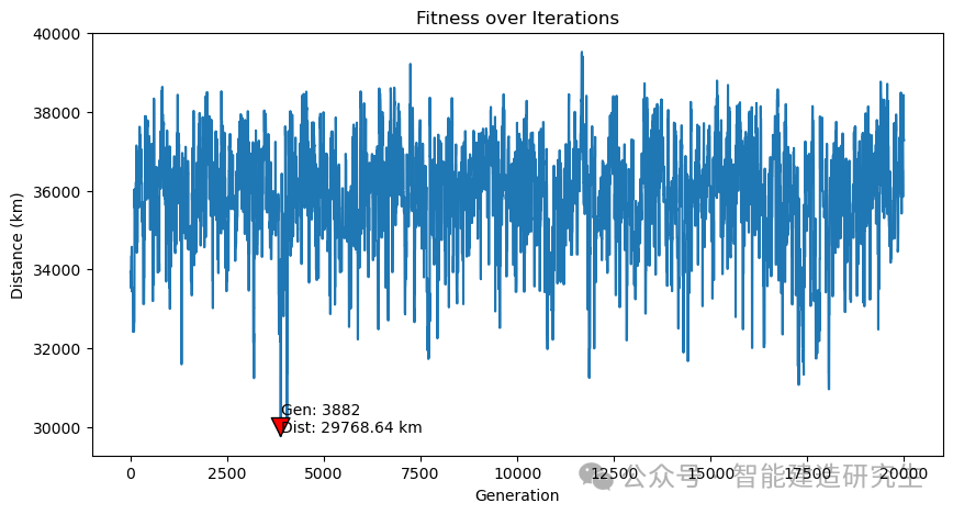
# 图2:适应度随迭代次数变化
fig2, ax2 = plt.subplots(figsize=(10, 5))
ax2.plot([x[1] for x in progress])
ax2.set_ylabel('Distance (km)')
ax2.set_xlabel('Generation')
ax2.set_title('Fitness over Iterations')
# 在图中标注最短距离和对应代数
ax2.annotate(f'Gen: {best_generation}\nDist: {best_distance:.2f} km',
xy=(best_generation, best_distance),
xytext=(best_generation, best_distance + 100),
arrowprops=dict(facecolor='red', shrink=0.05))
plt.show()
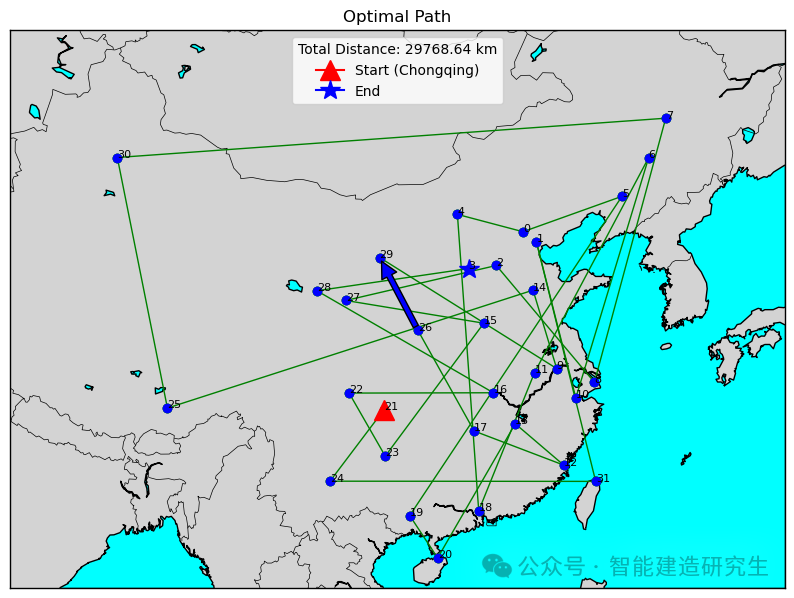
# 图3:显示最优路径
fig3, ax3 = plt.subplots(figsize=(10, 10))
m2 = Basemap(projection='merc', llcrnrlat=18, urcrnrlat=50, llcrnrlon=80, urcrnrlon=135, resolution='l', ax=ax3)
m2.drawcoastlines()
m2.drawcountries()
m2.fillcontinents(color='lightgray', lake_color='aqua')
m2.drawmapboundary(fill_color='aqua')
# 绘制最优路径和有向箭头
for i in range(len(best_route) - 1):
x1, y1 = m2(locations[best_route[i]][1], locations[best_route[i]][0])
x2, y2 = m2(locations[best_route[i + 1]][1], locations[best_route[i + 1]][0])
m2.plot([x1, x2], [y1, y2], color='g', linewidth=1, marker='o')
# 只添加一个代表方向的箭头
mid_index = len(best_route) // 2
mid_x1, mid_y1 = m2(locations[best_route[mid_index]][1], locations[best_route[mid_index]][0])
mid_x2, mid_y2 = m2(locations[best_route[mid_index + 1]][1], locations[best_route[mid_index + 1]][0])
ax3.annotate('', xy=(mid_x2, mid_y2), xytext=(mid_x1, mid_y1), arrowprops=dict(facecolor='blue', shrink=0.05))
# 在最优路径图上绘制城市位置
for i, (lat, lon) in enumerate(locations):
x, y = m2(lon, lat)
m2.plot(x, y, 'bo')
ax3.text(x, y, str(i), fontsize=8)
# 添加起点和终点标记
start_x, start_y = m2(locations[best_route[0]][1], locations[best_route[0]][0])
end_x, end_y = m2(locations[best_route[-1]][1], locations[best_route[-1]][0])
ax3.plot(start_x, start_y, marker='^', color='red', markersize=15, label='Start (Chongqing)') # 起点
ax3.plot(end_x, end_y, marker='*', color='blue', markersize=15, label='End') # 终点
# 添加总距离的图例
ax3.legend(title=f'Total Distance: {best_distance:.2f} km')
ax3.set_title('Optimal Path')
plt.show()
中国所有省会城市的位置可视化:
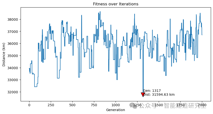
迭代次数为2千次(得到最短距离为31594公里):
找到历史迭代过程中最短的路径的迭代,并可视化该最短路径。
情况二:迭代次数为2万次(得到最短距离为29768公里)
找到历史迭代过程中最短的路径的迭代,并可视化该次迭代的最短路径。
以上内容总结自网络,如有帮助欢迎转发,我们下次再见!


![[数仓]四、离线数仓(Hive数仓系统-续)](https://i-blog.csdnimg.cn/direct/f44f79df3dd6403b8863003fa118deb5.png)