参考来源:https://www.bilibili.com/video/BV1nt411r7tj
1.数据质量分析
缺失值
异常值:箱线图
一致值(多数据源不一致)
2.图像可视化
占比:饼图、气泡图(2-5维)
波动图:折线图
门槛效应和边际递减:分析营销费用和流量价格
3.常见标签
1.性别分布:男女其它
2.地区分布:省份北上广深
3.年龄分布:80900010
4.数据特征
数值:数量、平均数、极差、标准差、方差、极值
分布规律:均匀分布、正太分布、长尾分布
可视化方法:柱状图、条形图、散点图、饼状图
5.pandas操作
读取数据
order_products = pd.read_csv("./instacart/order_products__prior.csv")
连表查询
tab1 = pd.merge(aisles, products, on=["aisle_id", "aisle_id"])
建立交叉表
table = pd.crosstab(tab3["user_id"], tab3["aisle"])
pca降维sk-learn
datanew=sklearn.decomposition.PCA(n_components=0.95).fit_transform(data)
6.数据预处理
6.1归一化
将数据压缩到0-1.让计算容易处理有不损失数据间大小占比
    # 1、获取数据
    data = pd.read_csv("dating.txt")
    data = data.iloc[:, :3]
    print("data:\n", data)

    # 2、实例化一个转换器类 压缩到2-3
    transfer = MinMaxScaler(feature_range=(2, 3))

    # 3、调用fit_transform
    data_new = transfer.fit_transform(data)
    print("data_new:\n", data_new)
6.2标准化(转换器)
(x-mean)/var。将数据转换到均值为0均差为1.减少异常值对整体数据产生差异少的特点。让数据易用于训练
fit:计算mean、var。transform:计算(x-mean)/var
    # 1、获取数据
    data = pd.read_csv("dating.txt")
    data = data.iloc[:, :3]
    print("data:\n", data)

    # 2、实例化一个转换器类
    transfer = StandardScaler()

    # 3、调用fit_transform
    data_new = transfer.fit_transform(data)
    print("data_new:\n", data_new)
6.3 方差降维
方差低的数据标签舍弃
def variance_demo():
    """
    过滤低方差特征
    :return:
    """
    # 1、获取数据
    data = pd.read_csv("factor_returns.csv")
    data = data.iloc[:, 1:-2]
    print("data:\n", data)

    # 2、实例化一个转换器类
    transfer = VarianceThreshold(threshold=10)

    # 3、调用fit_transform
    data_new = transfer.fit_transform(data)
    print("data_new:\n", data_new, data_new.shape)

    # 计算某两个变量之间的相关系数
    r1 = pearsonr(data["pe_ratio"], data["pb_ratio"])
    print("相关系数:\n", r1)
    r2 = pearsonr(data['revenue'], data['total_expense'])
    print("revenue与total_expense之间的相关性:\n", r2)
6.4 数据直接排除
data = data.query("x < 2.5 & x > 2 & y < 1.5 & y > 1.0")
6.5 时间戳转化日期、星期、小时
time_value = pd.to_datetime(data["time"], unit="s")
date = pd.DatetimeIndex(time_value)
data["day"] = date.day
data["weekday"] = date.weekday
data["hour"] = date.hour
6.6数据聚合
place_count = data.groupby("place_id").count()["row_id"]
data_final = data[data["place_id"].isin(place_count[place_count > 3].index.values)]
6.7缺失值处理
# 2、缺失值处理
# 1)替换-》np.nan
data = data.replace(to_replace="?", value=np.nan)
# 2)删除缺失样本
data.dropna(inplace=True)
#%%
data.isnull().any() # 不存在缺失值
7.数据建模(预估器)
7.1 knn:小数据<1000
交叉验证:将训练集分为n组,进行n次训练,每次选择其中一组用来验证结果,其它组用于训练。
网格搜索:让数据自己从给定的超参数中,选择出最好的超参数。比如k临近中,让算法自己找出最合适的k
    """
    用KNN算法对鸢尾花进行分类,添加网格搜索和交叉验证
    :return:
    """
    # 1)获取数据
    iris = load_iris()

    # 2)划分数据集
    x_train, x_test, y_train, y_test = train_test_split(iris.data, iris.target, random_state=22)

    # 3)特征工程:标准化
    transfer = StandardScaler()
    x_train = transfer.fit_transform(x_train)
    x_test = transfer.transform(x_test)

    # 4)KNN算法预估器
    estimator = KNeighborsClassifier()

    # 加入网格搜索与交叉验证
    # 参数准备
    param_dict = {"n_neighbors": [1, 3, 5, 7, 9, 11]}
    estimator = GridSearchCV(estimator, param_grid=param_dict, cv=10)
    estimator.fit(x_train, y_train)

    # 5)模型评估
    # 方法1:直接比对真实值和预测值
    y_predict = estimator.predict(x_test)
    print("y_predict:\n", y_predict)
    print("直接比对真实值和预测值:\n", y_test == y_predict)

    # 方法2:计算准确率
    score = estimator.score(x_test, y_test)
    print("准确率为:\n", score)

    # 最佳参数:best_params_
    print("最佳参数:\n", estimator.best_params_)
    # 最佳结果:best_score_
    print("最佳结果:\n", estimator.best_score_)
    # 最佳估计器:best_estimator_
    print("最佳估计器:\n", estimator.best_estimator_)
    # 交叉验证结果:cv_results_
    print("交叉验证结果:\n", estimator.cv_results_)
7.2 决策树(可视化)易理解
https://blog.csdn.net/liu_1314521/article/details/115638429
    """
    用决策树对鸢尾花进行分类
    :return:
    """
    # 1)获取数据集
    iris = load_iris()

    # 2)划分数据集
    x_train, x_test, y_train, y_test = train_test_split(iris.data, iris.target, random_state=22)

    # 3)决策树预估器
    estimator = DecisionTreeClassifier(criterion="entropy")
    estimator.fit(x_train, y_train)

    # 4)模型评估
    # 方法1:直接比对真实值和预测值
    y_predict = estimator.predict(x_test)
    print("y_predict:\n", y_predict)
    print("直接比对真实值和预测值:\n", y_test == y_predict)

    # 方法2:计算准确率
    score = estimator.score(x_test, y_test)
    print("准确率为:\n", score)

    # 可视化决策树
    export_graphviz(estimator, out_file="iris_tree.dot", feature_names=iris.feature_names)
朴素贝叶斯:特征相互独立+贝叶斯公式。给定条件下求的目标的概率值分布。应用文本分布
    """
    用朴素贝叶斯算法对新闻进行分类
    :return:
    """
    # 1)获取数据
    news = fetch_20newsgroups(subset="all")

    # 2)划分数据集
    x_train, x_test, y_train, y_test = train_test_split(news.data, news.target)

    # 3)特征工程:文本特征抽取-tfidf
    transfer = TfidfVectorizer()
    x_train = transfer.fit_transform(x_train)
    x_test = transfer.transform(x_test)

    # 4)朴素贝叶斯算法预估器流程
    estimator = MultinomialNB()
    estimator.fit(x_train, y_train)

    # 5)模型评估
    # 方法1:直接比对真实值和预测值
    y_predict = estimator.predict(x_test)
    print("y_predict:\n", y_predict)
    print("直接比对真实值和预测值:\n", y_test == y_predict)

    # 方法2:计算准确率
    score = estimator.score(x_test, y_test)
    print("准确率为:\n", score)

    return None
7.3 随机森林(多模型决策)
使用多个随机维度进行决策树建模,将多个预测结果求总数
from sklearn.ensemble import RandomForestClassifier
from sklearn.model_selection import GridSearchCV
#%%
estimator = RandomForestClassifier()
# 加入网格搜索与交叉验证
# 参数准备
param_dict = {"n_estimators": [120,200,300,500,800,1200], "max_depth": [5,8,15,25,30]}
estimator = GridSearchCV(estimator, param_grid=param_dict, cv=3)
estimator.fit(x_train, y_train)

# 5)模型评估
# 方法1:直接比对真实值和预测值
y_predict = estimator.predict(x_test)
print("y_predict:\n", y_predict)
print("直接比对真实值和预测值:\n", y_test == y_predict)

# 方法2:计算准确率
score = estimator.score(x_test, y_test)
print("准确率为:\n", score)

# 最佳参数:best_params_
print("最佳参数:\n", estimator.best_params_)
# 最佳结果:best_score_
print("最佳结果:\n", estimator.best_score_)
# 最佳估计器:best_estimator_
print("最佳估计器:\n", estimator.best_estimator_)
# 交叉验证结果:cv_results_
print("交叉验证结果:\n", estimator.cv_results_)
7.4 线性回归
使用梯度下降寻找最小值。实际不会那么简单,这里主要用于理解原理
    # 1)获取数据
    boston = load_boston()
    print("特征数量:\n", boston.data.shape)

    # 2)划分数据集
    x_train, x_test, y_train, y_test = train_test_split(boston.data, boston.target, random_state=22)

    # 3)标准化
    transfer = StandardScaler()
    x_train = transfer.fit_transform(x_train)
    x_test = transfer.transform(x_test)

    # 4)预估器
    estimator = SGDRegressor(learning_rate="constant", eta0=0.01, max_iter=10000, penalty="l1")
    estimator.fit(x_train, y_train)

    # 5)得出模型
    print("梯度下降-权重系数为:\n", estimator.coef_)
    print("梯度下降-偏置为:\n", estimator.intercept_)

    # 6)模型评估
    y_predict = estimator.predict(x_test)
    print("预测房价:\n", y_predict)
    error = mean_squared_error(y_test, y_predict)
    print("梯度下降-均方误差为:\n", error)
随机梯度下降(sag)解决直接梯度下降迭代慢,和随机梯度下降不准确的确定。使用随机数的平均值来在两者取平均。
7.4.2过拟合解决(岭回归)
欠拟合:特征数量不够,或数据集不够
过拟合:特征数量过多,数据集不够。解决:正则化,将高阶项进行惩罚。
岭回归:线性回归+L2正则
   """
    岭回归对波士顿房价进行预测
    :return:
    """
    # 1)获取数据
    boston = load_boston()
    print("特征数量:\n", boston.data.shape)

    # 2)划分数据集
    x_train, x_test, y_train, y_test = train_test_split(boston.data, boston.target, random_state=22)

    # 3)标准化
    transfer = StandardScaler()
    x_train = transfer.fit_transform(x_train)
    x_test = transfer.transform(x_test)

    # 4)预估器
    # estimator = Ridge(alpha=0.5, max_iter=10000)
    # estimator.fit(x_train, y_train)

    # 保存模型
    # joblib.dump(estimator, "my_ridge.pkl")
    # 加载模型
    estimator = joblib.load("my_ridge.pkl")

    # 5)得出模型
    print("岭回归-权重系数为:\n", estimator.coef_)
    print("岭回归-偏置为:\n", estimator.intercept_)

    # 6)模型评估
    y_predict = estimator.predict(x_test)
    print("预测房价:\n", y_predict)
    error = mean_squared_error(y_test, y_predict)
    print("岭回归-均方误差为:\n", error)
7.4.3逻辑回归
逻辑回归:线性回归的输入+sigmo压缩到01,将0.5作为二分类的分界线
损失函数:对数似然函数,将接近1的数损失越少,接近0损失越大。
7.5自动聚类
没有目标值,单单纯想先分类,在对数据进行预测训练
# 预估器流程
from sklearn.cluster import KMeans
#%%
estimator = KMeans(n_clusters=3)
estimator.fit(data_new)
#%%
y_predict = estimator.predict(data_new)
#%%
y_predict[:300]
#%%
# 模型评估-轮廓系数
from sklearn.metrics import silhouette_score
#%%
silhouette_score(data_new, y_predict)
8.模型评估
精确率:查的准不准
召回率:查的全不全
# 查看精确率、召回率、F1-score
from sklearn.metrics import classification_report
report = classification_report(y_test, y_predict, labels=[2, 4], target_names=["良性", "恶性"])
print(report)
roc: 随机:召回率=漏放率=0.5 准确:召回率=1
from sklearn.metrics import roc_auc_score
roc_auc_score(y_true, y_predict)
模型保存和加载
# 保存模型# joblib.dump(estimator, "my_ridge.pkl")
# 加载模型estimator = joblib.load("my_ridge.pkl")
附录
1.jupyter学习
conda create -n mylab python=3.11
conda activate mylab
python -m pip install --upgrade pip
pip install jupyterlab
jupyter lab .
快捷键
创建下一行: Alt+Enter
删除当前行 esc dd 清空当前行ctrl d
2.安装代码提示
pip3 install jupyter-lsp
pip install python-language-server[all]
插件搜索lsp
设置中搜索 completion开启两个自动补全