1.卷积神经网络CNN完成分类
1.1导入模块和数据
import tensorflow as tf
from tensorflow.keras import datasets, layers, models
import matplotlib.pyplot as plt

(train_images, train_labels),(test_images, test_labels)=datasets.fashion_mnist.load_data()

fashion = tf.keras.datasets.fashion_mnist
(train_x,train_y),(test_x,test_y) = fashion.load_data() # 可以直接调用 tf.keras.datasets.fashion_mnist,直接下载数据集
print('\n train_x:%s, train_y:%s, test_x:%s, test_y:%s'%(train_x.shape,train_y.shape,test_x.shape,test_y.shape))
train_x:(60000, 28, 28), train_y:(60000,), test_x:(10000, 28, 28), test_y:(10000,)
1.2 数据归一化
将像素的值标准化到[0,1]区间内
train_images&train_labels是训练集,模型用于学习
test_iamges&test_labels是测试集,用于测试
X_train,X_test = tf.cast(train_images/255.0,tf.float32),tf.cast(test_images/255.0,tf.float32)     #归一化
y_train,y_test = tf.cast(train_labels,tf.int16),tf.cast(test_labels,tf.int16)

train_images, test_images=train_images/255.0, test_images/255.0

train_images.shape, test_images.shape, train_labels.shape, test_labels.shape
((60000, 28, 28), (10000, 28, 28), (60000,), (10000,))
1.3 调整图片格式
train_images=train_images.reshape((60000,28,28,1))
test_images=test_images.reshape((10000,28,28,1))

train_images.shape, test_images.shape
#(batch_size, height, width, channels)
((60000, 28, 28, 1), (10000, 28, 28, 1))
1.4 可视化
class_names=['T-shirt/top', 'Trouser', 'Pullover', 'Dress', 'Coat', 'Sandal', 'Shirt', 'Sneaker', 'Bag', 'ankle boot']

plt.figure(figsize=(20,10))
for i in range(60):
  plt.subplot(5,12,i+1)
  plt.xticks([])
  plt.yticks([])
  plt.grid(False)
  plt.imshow(train_images[i], cmap=plt.cm.binary)
  plt.xlabel(class_names[train_labels[i]])
plt.show()

1.5 构建CNN网络
model=models.Sequential([
    layers.Conv2D(32,(3,3), activation='relu', input_shape=(28,28,1)),  #卷积层1,卷积核3X3
    layers.MaxPooling2D((2,2)),          #池化层1,2X2采样
    layers.Conv2D(64,(3,3), activation='relu',), #卷积层2,卷积核3X3
    layers.MaxPooling2D((2,2)),          #池化层1,2X2采样
    layers.Conv2D(32,(3,3), activation='relu', input_shape=(28,28,1)),  #卷积层1,卷积核3X3

    layers.Flatten(), #Flatten层,连接卷积层与全连接层
    layers.Dense(64, activation='relu'), #全连接层,特征进一步提取
    layers.Dense(10)
])

model.summary()  #打印网络结构
Model: "sequential_3"
_________________________________________________________________
 Layer (type)                Output Shape              Param #
=================================================================
 conv2d_9 (Conv2D)           (None, 26, 26, 32)        320

 max_pooling2d_6 (MaxPoolin  (None, 13, 13, 32)        0
 g2D)

 conv2d_10 (Conv2D)          (None, 11, 11, 64)        18496

 max_pooling2d_7 (MaxPoolin  (None, 5, 5, 64)          0
 g2D)

 conv2d_11 (Conv2D)          (None, 3, 3, 32)          18464

 flatten_3 (Flatten)         (None, 288)               0

 dense_6 (Dense)             (None, 64)                18496

 dense_7 (Dense)             (None, 10)                650

=================================================================
Total params: 56426 (220.41 KB)
Trainable params: 56426 (220.41 KB)
Non-trainable params: 0 (0.00 Byte)
_________________________________________________________________
1.6 编译
损失函数(loss):用于测量模型在训练期间的准确率。您会希望最小化此函数,以便将模型“引导”到正确的方向上。
优化器(optimizer):决定模型如何根据其看到的数据和自身的损失函数进行更新。
指标(metrics):用于监控训练和测试步骤。以下示例使用了准确率,即被正确分类的图像的比率。
model.compile( optimizer='adam',
        loss=tf.keras.losses.SparseCategoricalCrossentropy(from_logits=True),
        metrics=['accuracy']
)
1.7 训练模型
history=model.fit(train_images, train_labels,epochs=10,validation_data=(test_images, test_labels))

history2 = model.fit(X_train,y_train,batch_size=64,epochs=5,validation_split=0.2)
Epoch 1/10
1875/1875 [==============================] - 9s 4ms/step - loss: 0.5253 - accuracy: 0.8069 - val_loss: 0.3884 - val_accuracy: 0.8580
Epoch 2/10
1875/1875 [==============================] - 8s 4ms/step - loss: 0.3390 - accuracy: 0.8765 - val_loss: 0.3217 - val_accuracy: 0.8857
Epoch 3/10
1875/1875 [==============================] - 7s 4ms/step - loss: 0.2907 - accuracy: 0.8935 - val_loss: 0.2955 - val_accuracy: 0.8943
Epoch 4/10
1875/1875 [==============================] - 8s 4ms/step - loss: 0.2595 - accuracy: 0.9049 - val_loss: 0.2789 - val_accuracy: 0.9014
Epoch 5/10
1875/1875 [==============================] - 7s 4ms/step - loss: 0.2362 - accuracy: 0.9131 - val_loss: 0.2810 - val_accuracy: 0.8978
Epoch 6/10
1875/1875 [==============================] - 8s 4ms/step - loss: 0.2170 - accuracy: 0.9202 - val_loss: 0.2855 - val_accuracy: 0.8988
Epoch 7/10
1875/1875 [==============================] - 8s 4ms/step - loss: 0.2020 - accuracy: 0.9248 - val_loss: 0.2804 - val_accuracy: 0.8944
Epoch 8/10
1875/1875 [==============================] - 7s 4ms/step - loss: 0.1885 - accuracy: 0.9305 - val_loss: 0.2640 - val_accuracy: 0.9080
Epoch 9/10
1875/1875 [==============================] - 9s 5ms/step - loss: 0.1730 - accuracy: 0.9345 - val_loss: 0.2747 - val_accuracy: 0.9067
Epoch 10/10
1875/1875 [==============================] - 7s 4ms/step - loss: 0.1648 - accuracy: 0.9383 - val_loss: 0.2773 - val_accuracy: 0.9067
Epoch 1/5
750/750 [==============================] - 4s 4ms/step - loss: 0.1294 - accuracy: 0.9532 - val_loss: 0.1319 - val_accuracy: 0.9481
Epoch 2/5
750/750 [==============================] - 3s 4ms/step - loss: 0.1204 - accuracy: 0.9562 - val_loss: 0.1371 - val_accuracy: 0.9490
Epoch 3/5
750/750 [==============================] - 3s 4ms/step - loss: 0.1137 - accuracy: 0.9583 - val_loss: 0.1565 - val_accuracy: 0.9391
Epoch 4/5
750/750 [==============================] - 4s 5ms/step - loss: 0.1087 - accuracy: 0.9599 - val_loss: 0.1449 - val_accuracy: 0.9465
Epoch 5/5
750/750 [==============================] - 3s 4ms/step - loss: 0.1023 - accuracy: 0.9614 - val_loss: 0.1605 - val_accuracy: 0.9433
1.8预测
plt.imshow(test_images[1])
<matplotlib.image.AxesImage at 0x7e10dc8aa5c0>

import numpy as np

pre=model.predict(test_images)
print(class_names[np.argmax(pre[1])])
313/313 [==============================] - 1s 2ms/step
Pullover
1.9模型评估
plt.plot(history.history['accuracy'], label='accuracy')
plt.plot(history.history['val_accuracy'], label = 'val_accuracy')
plt.xlabel('Epoch')
plt.ylabel('Accuracy')
plt.ylim([0.5, 1])
plt.legend(loc='lower right')
plt.show()

test_loss, test_acc = model.evaluate(test_images,  test_labels, verbose=2)

313/313 - 1s - loss: 0.3033 - accuracy: 0.9113 - 598ms/epoch - 2ms/step
print("测试准确率为:",test_acc)
测试准确率为: 0.911300003528595
plt.figure(figsize=(10,3))

plt.subplot(121)
plt.plot(loss,color='b',label='train')
plt.plot(val_loss,color='r',label='test')
plt.ylabel('loss')
plt.legend()

plt.subplot(122)
plt.plot(acc,color='b',label='train')
plt.plot(val_acc,color='r',label='test')
plt.ylabel('Accuracy')
plt.legend()

#暂停5秒关闭画布,否则画布一直打开的同时,会持续占用GPU内存
#根据需要自行选择
#plt.ion()       #打开交互式操作模式
#plt.show()
#plt.pause(5)
#plt.close()
<matplotlib.legend.Legend at 0x7e10dc23f640>

1.10 保存模型
#保存整个模型
model.save('fashion_CNN_weights.h5')
/usr/local/lib/python3.10/dist-packages/keras/src/engine/training.py:3103: UserWarning: You are saving your model as an HDF5 file via `model.save()`. This file format is considered legacy. We recommend using instead the native Keras format, e.g. `model.save('my_model.keras')`.
  saving_api.save_model(
#使用模型
plt.figure()
for i in range(10):
    num = np.random.randint(1,10000)

    plt.subplot(2,5,i+1)
    plt.axis('off')
    plt.imshow(test_images[num],cmap='gray')
    demo = tf.reshape(X_test[num],(1,28,28,1)  # 查看train和test在reshape后的大小
    y_pred = np.argmax(model.predict(demo))
    plt.title('label:'+str(test_y[num])+'\n predict:'+str(y_pred))
#y_pred = np.argmax(model.predict(X_test[0:5]),axis=1)
#print('X_test[0:5]: %s'%(X_test[0:5].shape))
#print('y_pred: %s'%(y_pred))

#plt.ion()       #打开交互式操作模式
plt.show()
#plt.pause(5)
#plt.close()
1/1 [==============================] - 0s 302ms/step
1/1 [==============================] - 0s 37ms/step
1/1 [==============================] - 0s 16ms/step
1/1 [==============================] - 0s 16ms/step
1/1 [==============================] - 0s 16ms/step
1/1 [==============================] - 0s 20ms/step
1/1 [==============================] - 0s 16ms/step
1/1 [==============================] - 0s 16ms/step
1/1 [==============================] - 0s 16ms/step
1/1 [==============================] - 0s 16ms/step