pytorch中创建maskrcnn模型

0.模型输入/输出参数参见

链接: pytorch的mask-rcnn的模型参数解释
核心代码
GeneralizedRCNN(这里以mask-rcnn来解释说明)

# 通过输入图像获取fpn特征图,注意这里的backbone不是直接的resnet,而是fpn化后的
features = self.backbone(images.tensors)
# 由于是mask-rcnn,故而是一个dict,这里是处理非fpn的包装为dict
if isinstance(features, torch.Tensor):
    features = OrderedDict([("0", features)])
# RPN负责生成候选区域（proposals）。它基于前面提取的特征features，以及输入图像images和目标targets（如果有的话，例如在训练阶段）来生成这些候选区域。同时，它也可能返回与候选区域生成相关的损失proposal_losses。
proposals, proposal_losses = self.rpn(images, features, targets)
#ROI Heads（Region of Interest Heads）负责对这些候选区域进行分类和边界框回归。它基于RPN生成的候选区域proposals，前面提取的特征features，以及输入图像的大小images.image_sizes和目标targets来执行这些任务。同时，它返回检测结果detections和与分类和边界框回归相关的损失detector_losses。
detections, detector_losses = self.roi_heads(features, proposals, images.image_sizes, targets)
# 后处理步骤通常包括将检测结果从模型输出格式转换为更易于解释或可视化的格式。例如，它可能包括将边界框坐标从模型使用的格式转换为图像的实际像素坐标，或者对分类得分进行阈值处理以过滤掉低置信度的检测。
detections = self.transform.postprocess(detections, images.image_sizes, original_image_sizes)  # type: ignore[operator]
# 汇总损失
losses = {}
losses.update(detector_losses)
losses.update(proposal_losses)

核心模型类:

MaskRCNN(FasterRCNN)
FasterRCNN(GeneralizedRCNN)
GeneralizedRCNN(nn.Module)
# 处理原始图像
GeneralizedRCNNTransform(nn.Module)
BackboneWithFPN(nn.Module)
IntermediateLayerGetter(nn.ModuleDict)
FeaturePyramidNetwork(nn.Module)
# RPN网络
RegionProposalNetwork(nn.Module)
# 建立anchor
AnchorGenerator(nn.Module)
# rpnhead
RPNHead(nn.Module)

1.提取特征图

通过骨干网络（如ResNet）提取输入图像的特征图

1.1 执行transform

对输入的images,targets执行transform,主要是标准化和resize的合并操作

1.1.1 images执行标准化操作

如果是采用的imagenet权重,则一般采用以下参数执行标准化操作.主要作用屏蔽图像色温/曝光一类的影响.
注意,传入到模型的images是0-1之间的float表示的tensor

image_mean = [0.485, 0.456, 0.406]
image_std = [0.229, 0.224, 0.225]

1.1.2 images执行resize操作

同一个batch的图像需要缩放到同一尺寸,才可以合并.
定义dataloader时的sampler,可以创建一个相似宽高比的图像分配到一组组成batch的sapmler以优化计算.
模型需要指定一个max_size以及一个min_size.过大/小的图像会被缩放至一个合适尺寸.
resize方法可以采用双线性插值法(pytorch的模型是这么干的),或者直接填充.

1.1.3targets的mask执行resize操作

图像resize了,mask也需要同样操作,不然对不上.方法和图像的一致

1.1.4 images执行合并tensor操作

将list(tensor([N,H,W]))[B] 合并为tensor[B,N,H,W]以便传入backbone

1.2 创建backbone,以及backbone_with_fpn

1.2.1 使用backbone网络,提取创建fpn网络

例如restnet50,不需要返回分类信息,而是前面的多层特征图信息,然后组合为fpn数据
调用栈
GeneralizedRCNN.forward->
RegionProposalNetwork.forward->
BackboneWithFPN.forward

backbone = resnet50(weights=weights_backbone, progress=progress, norm_layer=norm_layer)
backbone = _resnet_fpn_extractor(backbone, trainable_backbone_layers)

输出结果形如:

1.2.2 提取fpn特征数据

现在我们来提取输出features
一共分2步,body和fpn
body从backbone提取原始特征层数据 (pytorch 定义为 IntermediateLayerGetter 类)
fpn将其处理打包为fpn结构数据 (pytorch 定义为 FeaturePyramidNetwork 类)

def forward(self, x: Tensor) -> Dict[str, Tensor]:
     x = self.body(x)
     x = self.fpn(x)
     return x

1.2.2.1 body

resnet的网络结构如下,我们需要提取layer1-4的输出结果来构建fpn,
提取所有return_layers最后一个层,即layer4之前的所有层,即抛弃掉无用的avgpool和fc层

参考精简代码如下:

import copy
from collections import OrderedDict

import torch
from PIL import Image
from torchvision.models import resnet50, ResNet50_Weights
from torchvision import transforms

if __name__ == '__main__':
    model = resnet50(weights=ResNet50_Weights.DEFAULT)
    original_img = Image.open("a.png").convert('RGB')
    ts = transforms.Compose([transforms.ToTensor()])
    img = ts(original_img)
    img = torch.unsqueeze(img, dim=0)
    model.eval()

    # 需要返回用以构建fpn层的名字
    return_layers = {'layer1': '0', 'layer2': '1', 'layer3': '2', 'layer4': '3'}
    # 创建return_layers的副本
    return_layers_copy = copy.deepcopy(return_layers)
    # 存储有效的层
    layers = OrderedDict()
    # 提取所有return_layers最后一个层,即layer4之前的所有层,即抛弃掉无用的avgpool和fc层
    for name, module in model.named_children():
        layers[name] = module
        if name in return_layers_copy:
            del return_layers_copy[name]
        # 如果指示的层被删光了,说明遍历到最后一个了,跳出循环
        if not return_layers_copy:
            break
    # 创建结果集合
    out = OrderedDict()
    for name, module in layers.items():
        img = module(img)
        if name in return_layers:
            out_name = return_layers[name]
            out[out_name] = img
    # rs = model(img)
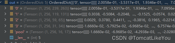
    print(out)

输出入下图

1.2.2.2 fpn

对body输出的out的4个结果分别执行1x1的卷积操作(共4个卷积核,输出均为256,输入是256~2048)得到结果
精简代码如下:

o2 = list()
in_channels_list = [256, 512, 1024, 2048]
out_channels = 256
# 使用一个1x1的卷积核处理为同样深度的特征图
inner_blocks = nn.ModuleList()
for index, in_channels in enumerate(in_channels_list):
	inner_block_module = nn.Conv2d(in_channels, out_channels, kernel_size=1, padding=0)
	inner_blocks.append(inner_blocks)
	# 等效于不设定激活函数和归一化层的Conv2d,注意Conv2dNormActivation会自动计算padding,以使之尺寸不变
	# inner_block_module2 = Conv2dNormActivation(in_channels, out_channels, kernel_size=1, padding=0, norm_layer=None,
	#                                            activation_layer=None)
	x = out.get(str(index))
	x = inner_block_module(x)
	o2.append(x)

 print(o2)

输出如下
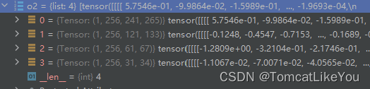对同一深度的结果(o2)操作上采样以及相加,即:
注:此处方便理解,C代表代码中的o2,C2代表o2的下标2,所以有0,和论文中的不太一致
C3=P3
P3上采样+C2=P2
P2上采样+C1=P1
P1上采样+C0=P0

对P0-3分别做一次3x3的卷积,对P3做最大池化得pool
P0->3x3卷积=out(0)
P1->3x3卷积=out(1)
P2->3x3卷积=out(2)
P3->3x3卷积=out(3)
P3->maxpool=pool
代码简化示意如下:

 # 执行上采样以及合并操作,以及结果再次卷积
    o3 = list()
    # 最后一个直接丢到结果集上,作为p4
    last_inner = o2[-1]
    o3.append(last_inner)

    # 倒着遍历o2,从倒数第3个开始
    # 使用一个3x3的卷积核再次处理结果, 减少上采样的混叠效应
    layer_blocks = nn.ModuleList()
    for idx in range(len(o2) - 2, -1, -1):
        # 获取当前这个,以及形状
        inner_lateral = o2[idx]
        feat_shape = inner_lateral.shape[-2:]
        # 对上层的那个执行上采样
        inner_top_down = nn.functional.interpolate(last_inner, size=feat_shape)
        # 相加作为P3~P1
        last_inner = inner_lateral + inner_top_down

        # 使用一个3x3的卷积核再次处理结果,减少上采样的混叠效应
        layer_block_module = nn.Conv2d(out_channels, out_channels, kernel_size=3, padding=0)
        layer_blocks.append(layer_block_module)

        # 倒序存储到结果上
        o3.insert(0, layer_block_module(last_inner))

    # 取出最小特征图做一次池化,池化核1x1,步长2
    tm = nn.functional.max_pool2d(o3[-1], kernel_size=1, stride=2, padding=0)
    o3.append(tm)

    names = ["0", "1", "2", "3", "pool"]
    # make it back an OrderedDict
    out = OrderedDict([(k, v) for k, v in zip(names, o3)])
    print(o3)

以上全部演示代码

import copy
from collections import OrderedDict

import torch
from PIL import Image
from torchvision.models import resnet50, ResNet50_Weights
from torchvision import transforms
from torchvision.ops import Conv2dNormActivation
from torch import nn

if __name__ == '__main__':
    model = resnet50(weights=ResNet50_Weights.DEFAULT)
    original_img = Image.open("a.png").convert('RGB')
    ts = transforms.Compose([transforms.ToTensor()])
    img = ts(original_img)
    img = torch.unsqueeze(img, dim=0)
    model.eval()

    # 需要返回用以构建fpn层的名字
    return_layers = {'layer1': '0', 'layer2': '1', 'layer3': '2', 'layer4': '3'}
    # 创建return_layers的副本
    return_layers_copy = copy.deepcopy(return_layers)
    # 存储有效的层
    layers = OrderedDict()
    # 提取所有return_layers最后一个层,即layer4之前的所有层,即抛弃掉无用的avgpool和fc层
    for name, module in model.named_children():
        layers[name] = module
        if name in return_layers_copy:
            del return_layers_copy[name]
        # 如果指示的层被删光了,说明遍历到最后一个了,跳出循环
        if not return_layers_copy:
            break
    # 创建结果集合
    out = OrderedDict()
    for name, module in layers.items():
        img = module(img)
        if name in return_layers:
            out_name = return_layers[name]
            out[out_name] = img
    print(out)

    in_channels_list = [256, 512, 1024, 2048]
    out_channels = 256

    # 创建1x1卷积,并执行卷积操作
    o2 = list()
    # 使用一个1x1的卷积核处理为同样深度的特征图
    inner_blocks = nn.ModuleList()
    for index, in_channels in enumerate(in_channels_list):
        # 用以执行处理同一深度的卷积核
        inner_block_module = nn.Conv2d(in_channels, out_channels, kernel_size=1, padding=0)
        inner_blocks.append(inner_blocks)
        # 等效于不设定激活函数和归一化层的Conv2d
        # inner_block_module2 = Conv2dNormActivation(in_channels, out_channels, kernel_size=1, padding=0,
        #                                            norm_layer=None,activation_layer=None)
        x = out.get(str(index))
        x = inner_block_module(x)
        o2.append(x)

    # 执行上采样以及合并操作,以及结果再次卷积
    o3 = list()
    # 最后一个直接丢到结果集上,作为p4
    last_inner = o2[-1]
    o3.append(last_inner)

    # 倒着遍历o2,从倒数第3个开始
    # 使用一个3x3的卷积核再次处理结果, 减少上采样的混叠效应
    layer_blocks = nn.ModuleList()
    for idx in range(len(o2) - 2, -1, -1):
        # 获取当前这个,以及形状
        inner_lateral = o2[idx]
        feat_shape = inner_lateral.shape[-2:]
        # 对上层的那个执行上采样
        inner_top_down = nn.functional.interpolate(last_inner, size=feat_shape)
        # 相加作为P3~P1
        last_inner = inner_lateral + inner_top_down

        # 使用一个3x3的卷积核再次处理结果,减少上采样的混叠效应
        layer_block_module = nn.Conv2d(out_channels, out_channels, kernel_size=3, padding=0)
        layer_blocks.append(layer_block_module)

        # 倒序存储到结果上
        o3.insert(0, layer_block_module(last_inner))

    # 取出最小特征图做一次池化,卷积核1x1,步长2
    tm = nn.functional.max_pool2d(o3[-1], kernel_size=1, stride=2, padding=0)
    o3.append(tm)

    names = ["0", "1", "2", "3", "pool"]
    # make it back an OrderedDict
    out = OrderedDict([(k, v) for k, v in zip(names, o3)])
    print(o3)

在这个过程中,可以学习的参数分布在
1.backbone网络,可以锁定一些层不更新,pytorch默认是更新3个层
2.处理特征图为同一深度的1x1核的卷积层
3.最后输出前的3x3的卷积层

2 构建RPN网络

上文我们获取了5张尺寸各异,深度为256的特征图,下面我们对他进行RPN即
(Region Proposal Network)区域生成网络构建.
注意 : 后面的原图,均指被transform处理过的图像,而不是真的原原本本的图像

        features = self.backbone(images.tensors)
        if isinstance(features, torch.Tensor):
            features = OrderedDict([("0", features)])
        proposals, proposal_losses = self.rpn(images, features, targets)
        detections, detector_losses = self.roi_heads(features, proposals, images.image_sizes, targets)
        detections = self.transform.postprocess(detections, images.image_sizes, original_image_sizes)  # type: ignore[operator]

2.1 创建anchors

fpn创建了5张特征图(下图示例),我们取最大尺寸的为例,(其他的做法同理):

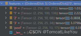
1. 特征图尺寸为: 1x256x200x272 (batch_size=1) ->记作A
2. 原始图像尺寸 800x1066 (实际尺寸为1848, 2464)->记作B
3. 可以看出 A的尺寸是B的4倍(大约) .
4. 做一个映射,一个A的点,映射到B上就是4个像素点.
5. 我给A的每一个点,创建9个候选框,长宽比为(0.5,1,2).长为(16,32,64)
6. 那么总计就是 200x272x9 = 489600个候选框.
7. 下面计算出每一个候选框的实际坐标,按照(x1,y1,x2,y2)返回一个(489600,4)的tensor

2.1.1 基础cell_anchor构建

8. 示例代码,计算出9个候选框的基础尺寸,其中scales代表是面积的开方,也可以理解为,在长宽比为1时,边长就是scales值.(注意实际使用的代码应该返回一个list,以适应5个特征图)
   调用栈
   GeneralizedRCNN.forward->
   RegionProposalNetwork.forward->
   AnchorGenerator.forward

import torch
from torch import Tensor


def generate_anchors(
        scales,
        aspect_ratios,
        dtype: torch.dtype = torch.float32,
        device: torch.device = torch.device("cpu"),
) -> Tensor:
    scales = torch.as_tensor(scales, dtype=dtype, device=device)
    aspect_ratios = torch.as_tensor(aspect_ratios, dtype=dtype, device=device)
    h_ratios = torch.sqrt(aspect_ratios)
    w_ratios = 1 / h_ratios

    ws = (w_ratios[:, None] * scales[None, :]).view(-1)
    hs = (h_ratios[:, None] * scales[None, :]).view(-1)

    base_anchors = torch.stack([-ws, -hs, ws, hs], dim=1) / 2
    return base_anchors.round()


if __name__ == '__main__':
    size = (16, 32, 64)
    aspect_ratio = (0.5, 1.0, 2.0)
    print(generate_anchors(size, aspect_ratio))

输出结果

tensor([[-11.,  -6.,  11.,   6.],
        [-23., -11.,  23.,  11.],
        [-45., -23.,  45.,  23.],
        [ -8.,  -8.,   8.,   8.],
        [-16., -16.,  16.,  16.],
        [-32., -32.,  32.,  32.],
        [ -6., -11.,   6.,  11.],
        [-11., -23.,  11.,  23.],
        [-23., -45.,  23.,  45.]])

2.1.2 计算中心点相加cell_anchor

9. 使用基础cell_anchor,A的所有点坐标,以及和原图的缩放关系,计算所有anchor.
   cell_anchor为(9x4),即A的每个点坐标都有9和候选框
   A尺寸为(200x272),即共有54400个坐标
   即最终结果应该是(54400x9x4) = (489600x4)的tensor
   其中4是由cell_anchor+缩放过比例的A坐标得到
   简化代码如下

import torch

from test2 import generate_anchors

if __name__ == '__main__':
    grid_height = 200
    grid_width = 272
    # 和原图的缩放比例
    stride_height = torch.tensor(4)
    stride_width = torch.tensor(4)
    device = torch.device("cpu")
    # 依照缩放比例,即步幅,将特征图像素点缩放到原始图上
    shifts_x = torch.arange(0, grid_width, dtype=torch.int32, device=device) * stride_width
    shifts_y = torch.arange(0, grid_height, dtype=torch.int32, device=device) * stride_height
    # 将(200x272)=54400个中心点数据(cx,cy) 变为54400x4的数据,即54400x(x1,y1,x2,y2)=(cx,cy,cx,cy)
    shift_y, shift_x = torch.meshgrid(shifts_y, shifts_x, indexing="ij")
    shift_x = shift_x.reshape(-1)
    shift_y = shift_y.reshape(-1)
    # shifts表示共有54400个中心点,每个中心点的坐标为(x1,y1,x2,y2);
    shifts = torch.stack((shift_x, shift_y, shift_x, shift_y), dim=1)
    # 获取cell_anchors(9,4) 表示每个中心点都有9中可能,坐标距离(x1,y1,x2,y2)偏移分别是(a1,b1,a2,b2)(例如:[-11.,  -6.,  11.,   6.])
    size = (16, 32, 64)
    aspect_ratio = (0.5, 1.0, 2.0)
    cell_anchor = generate_anchors(size, aspect_ratio)
    # 只需要将shifts(54400x4) + cell_anchors(9x4)相加即可的得到结果(489600x4),即shifts,cell_anchors的第一维分别扩展9和54400倍即可
    anchor = shifts.view(-1, 1, 4) + cell_anchor.view(1, -1, 4)
    # 将 54400x9x4 转为 489600x4 ,代表共有489600的anchor,每个含1个坐标(x1,y1,x2,y2)
    anchor = anchor.view(-1, 4)
    print(anchor.shape)

10. 对5个特征图执行相同操作,注意size的选用.在不同特征图上,size可以设置为不同形状的不同值,以适应在不同特征图尺寸的表现.
11. 分辨率越大的特征图,缩放比例就越小,中心点间距小,故而size的设定就应越小
12. 分辨率越小的特征图,缩放比例就越大,中心点间距大,故而size的设定就应越大
13. 例如size可以设定为((16, 32, 64),(32, 64, 128),(64,128,256),(128,256,512),(256,512,1024)),当然也可以设定为一样的,看需求如何,同理aspect_ratio 也可以按照实际的需求自行设定,比如存在细长棍状的物体时,可以比例设置为(0.25, 0.5, 1.0, 2.0, 4.0)
14. 按照每个scles=3.aspect_ratio =3来计算.总共获得个尺寸候选框分别为,最后加起来就好
    $$\begin{array}{rl}200\times 272\times 9& =489600\\ 100\times 136\times 9& =122400\\ 50\times 68\times 9& =30600\\ 25\times 34\times 9& =7650\\ 13\times 19\times 9& =2223\\ sum()& =652473\end{array}$$

2.2 计算每个anchor分类和回归值

这么多的候选框,首先进行一次判断,过绝大部分无用的anchor.

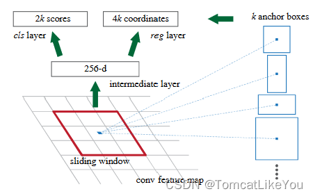
1. 需要判断这个anchor是否保留,即判断他存在物体的可能性有多高,例如设定可能性大于70%即保留.
2. 那这个存在物体就是一个二分类问题,即上图的2k scores
3. 预测框和实际物体边框(GT)的差距有多少,就是一个回归问题.即上图的4k coordinates
4. 注意,这个是需要对每一个候选框进行的操作

方案:
使用所有的特征图作为输入,创建一个模型RPNHead,计算预测,返回2个结果,分类结果与回归结果
即:使用一个3x3的卷积处理后分别接上分类卷积和回归卷积,输出通道数量应为每个点的可能的anchor数,即K,计算应得到2个结果
即
objectness(252473x1) = (
200x272x9x1+
100x136x9x1
…
)
pred_bbox_deltas (252473x4)= (
200x272x9x4+
100x136x9x4
…
)
注意 pred_bbox_deltas 并不是直接返回的直接边界值,而是和GT的偏差,因为图像尺寸不同原因,且是参数化后值,故有_deltas后缀
模型代码如下
调用栈
GeneralizedRCNN.forward->
RegionProposalNetwork.forward->
RPNHead.forward

class RPNHead(nn.Module):
    def __init__(self, in_channels: int, num_anchors: int, conv_depth=1) -> None:
        super().__init__()
        convs = []
        for _ in range(conv_depth):
            convs.append(Conv2dNormActivation(in_channels, in_channels, kernel_size=3, norm_layer=None))
        self.conv = nn.Sequential(*convs)
        self.cls_logits = nn.Conv2d(in_channels, num_anchors, kernel_size=1, stride=1)
        self.bbox_pred = nn.Conv2d(in_channels, num_anchors * 4, kernel_size=1, stride=1)

        for layer in self.modules():
            if isinstance(layer, nn.Conv2d):
                torch.nn.init.normal_(layer.weight, std=0.01)  # type: ignore[arg-type]
                if layer.bias is not None:
                    torch.nn.init.constant_(layer.bias, 0)  # type: ignore[arg-type]

		# 省略若干方法
    def forward(self, x: List[Tensor]) -> Tuple[List[Tensor], List[Tensor]]:
        logits = []
        bbox_reg = []
        for feature in x:
            t = self.conv(feature)
            logits.append(self.cls_logits(t))
            bbox_reg.append(self.bbox_pred(t))
        return logits, bbox_reg

2.3过滤无用候选框