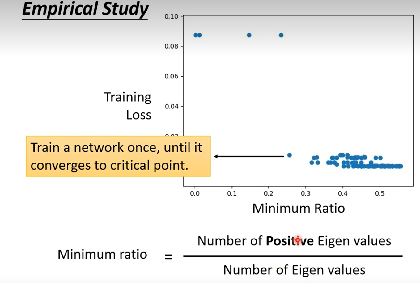
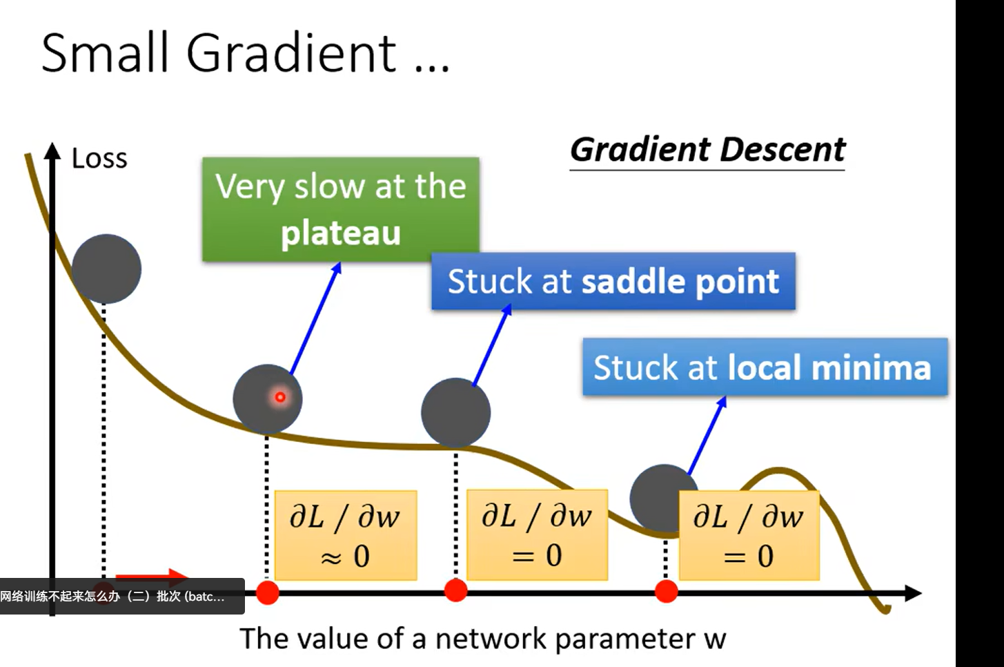
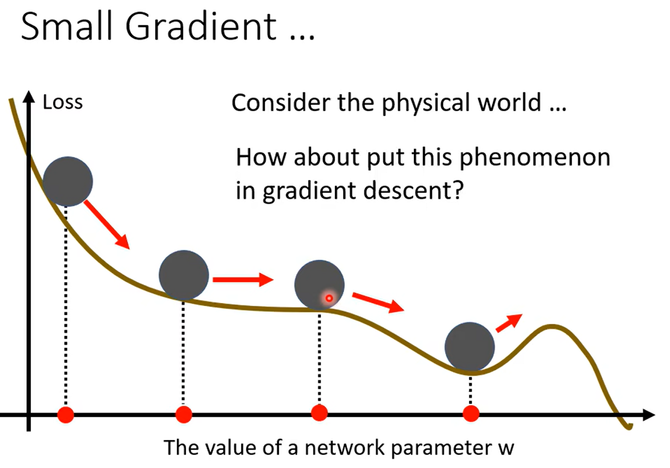
Day11 when gradient is small……
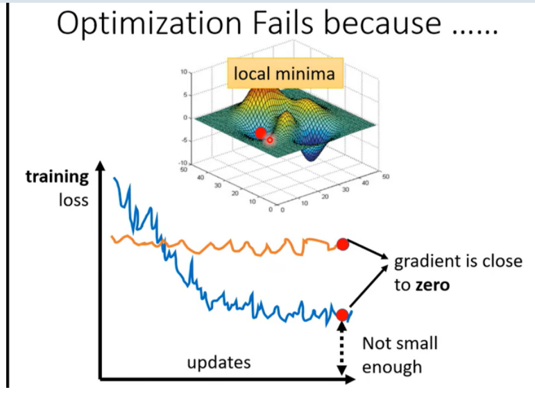
![image-20240411165229093](https://img-home.csdnimg.cn/images/20230724024159.png?origin_url=https%3A%2F%2Fmarkdown-pictures-jhx.oss-cn-beijing.aliyuncs.com%2Fpicgo%2Fimage-20240411165229093.png&pos_id=img-ZTBJKn2k-1712838404390%29)
![image-20240411170420173](https://img-home.csdnimg.cn/images/20230724024159.png?origin_url=https%3A%2F%2Fmarkdown-pictures-jhx.oss-cn-beijing.aliyuncs.com%2Fpicgo%2Fimage-20240411170420173.png&pos_id=img-QHta1FoL-1712838405043%29)
怎么知道是局部小 还是鞍点?
using Math
![image-20240411170714889](https://img-home.csdnimg.cn/images/20230724024159.png?origin_url=https%3A%2F%2Fmarkdown-pictures-jhx.oss-cn-beijing.aliyuncs.com%2Fpicgo%2Fimage-20240411170714889.png&pos_id=img-SzSc21Qe-1712838405767%29)
![image-20240411170827423](https://img-blog.csdnimg.cn/img_convert/333e28be0cb776c97491213a07b5e158.png)
![image-20240411183651821](https://img-blog.csdnimg.cn/img_convert/99e2f0d2bed2cdf4920a45f0481edac5.png)
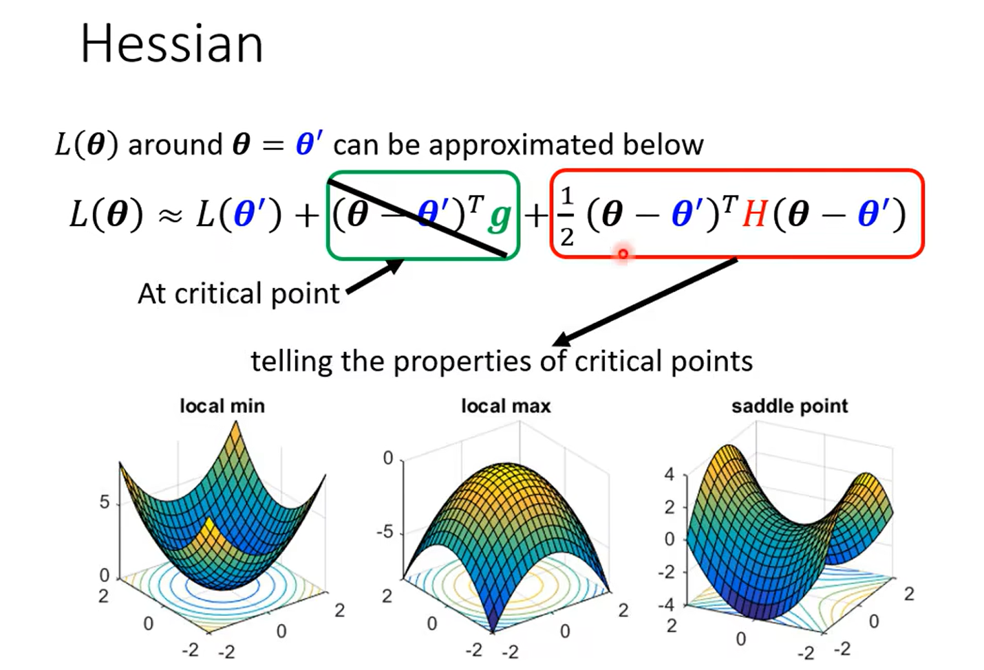
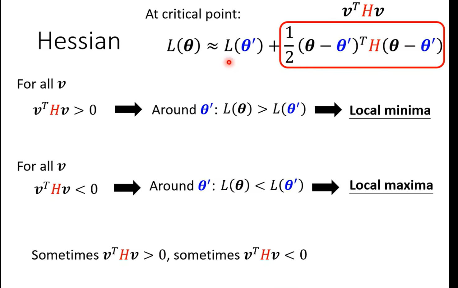
这里巧妙的说明了hessan矩阵可以决定一个二次函数的凹凸性 也就是 θ \theta θ 是min 还是max,最后那个有些有些 哈 是一个saddle;
然后这里只要看hessan矩阵是不是正定的就好(详见 线性代数)
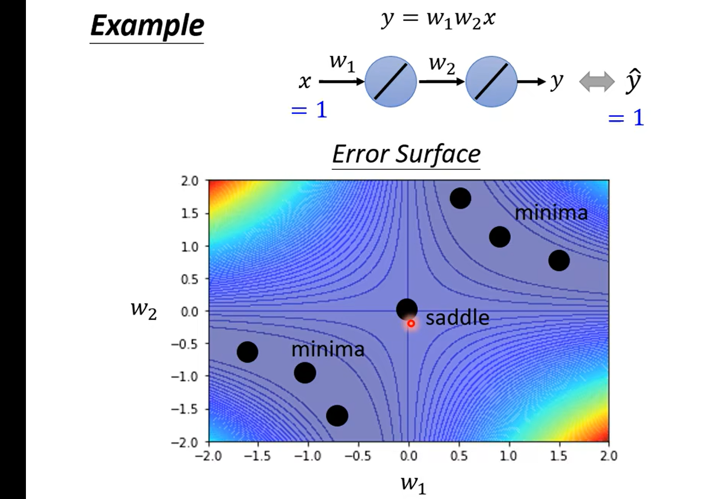
example – using Hessan
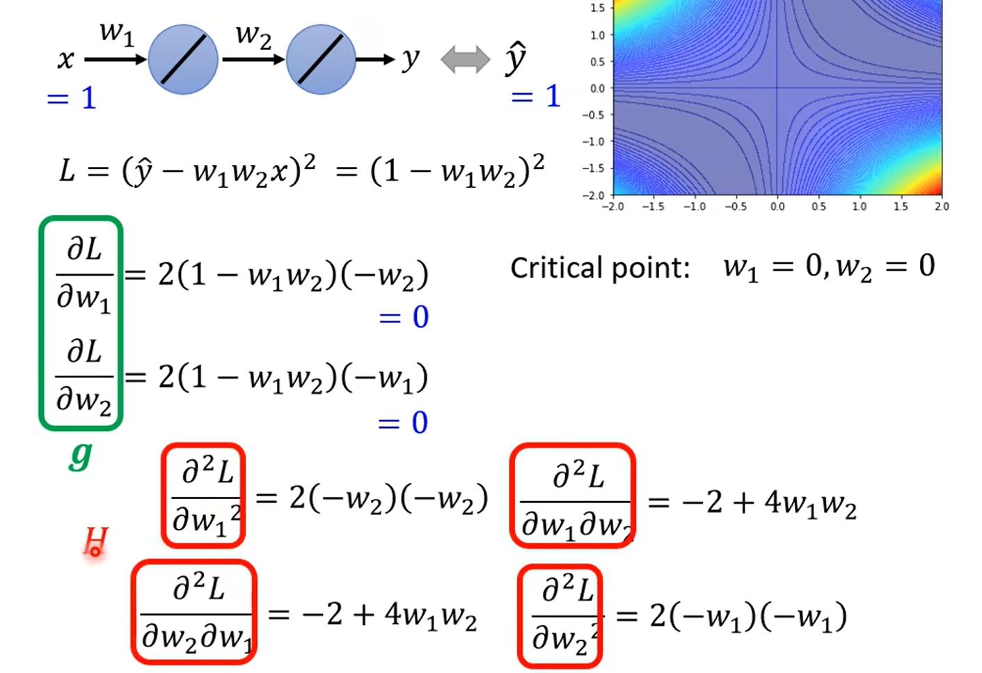
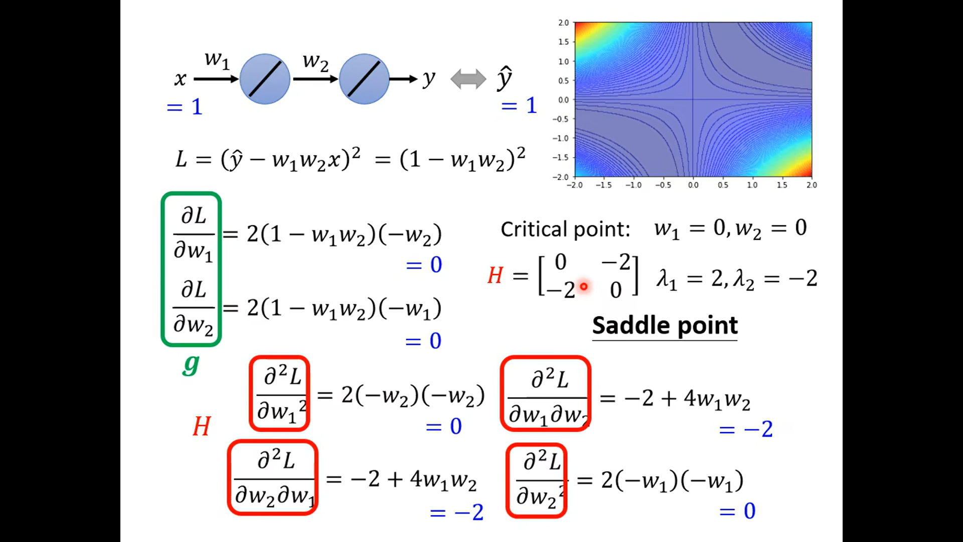
奇怪这里为什么不是主对角线呀,难道两个都一样嘛 晕死,得复习线代了
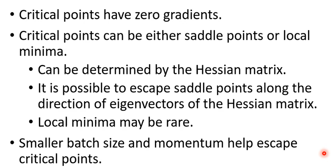
Dont afraid of saddle point(鞍点)
![image-20240411191229522](https://img-blog.csdnimg.cn/img_convert/a5df935e1d9a9dca10abcf1e230e0094.png)
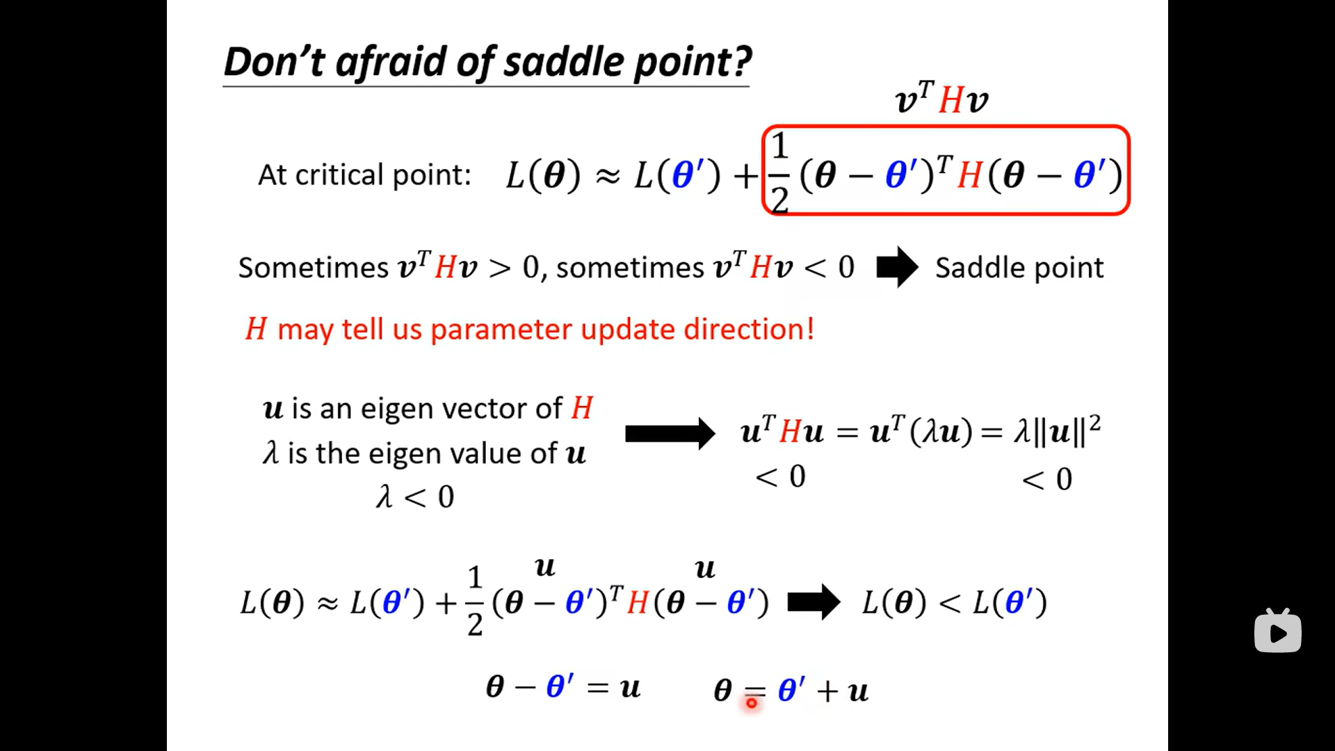
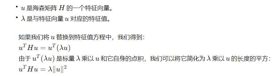
征向量 u 和对应的特征值 λ定义为满足下列关系的向量和标量:Hu=λu
在梯度下降算法中,我们希望选择使得 L*(*θ) 减小的 θ 方向。如果 λ<0,则向 u 的方向移动参数 θ 会减小损失函数 L(θ)。
换句话说,如果我们发现了一个负特征值λ 和相应的特征向量u,我们可以通过沿着 u 的方向更新 θ 来降低损失函数的值。这就是图中所说的“Decrease L”的含义。
![image-20240411192321757](https://img-blog.csdnimg.cn/img_convert/2104332666d98e0690bf4299c9fd7c0c.png)
local minima VS saddle Point
![image-20240411193129424](https://img-blog.csdnimg.cn/img_convert/4a73440fbfa2638d79eff804b1efdc33.png)
![image-20240411193238944](https://img-blog.csdnimg.cn/img_convert/7d59169704d7d30fc2150404459f1e1d.png)
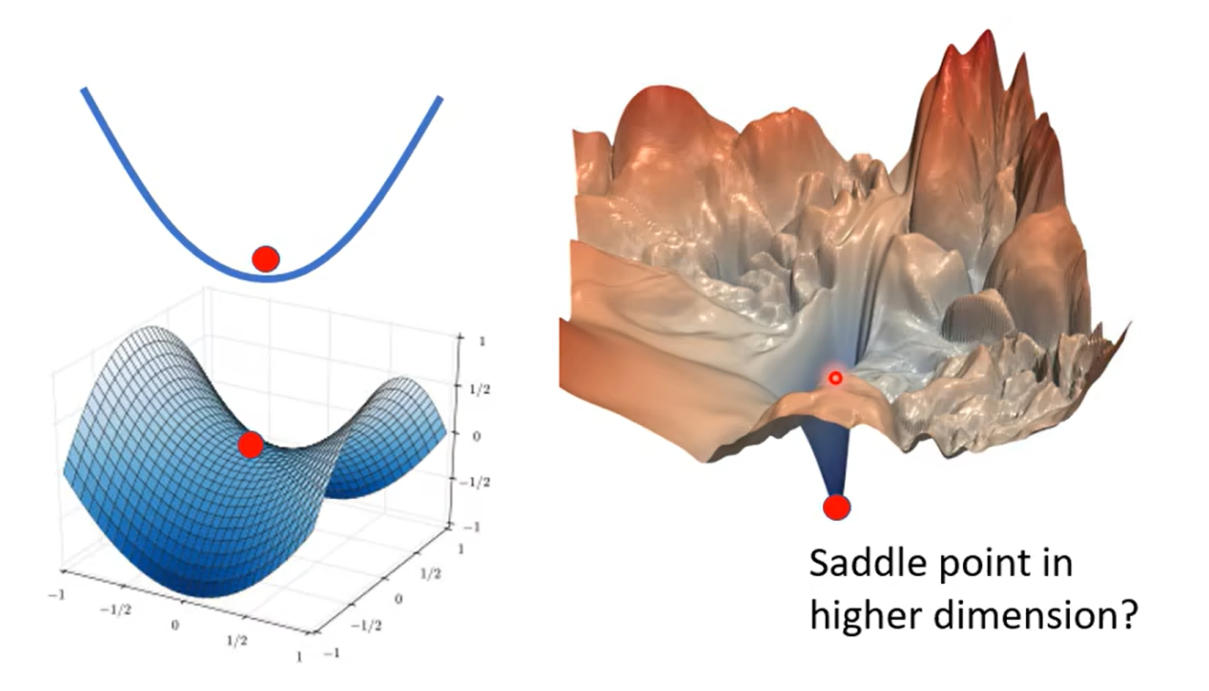
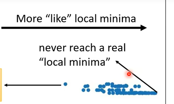
引入高维空间的观点,解决local minima的问题:我们很少遇到local minima;
![image-20240411193304041](https://img-blog.csdnimg.cn/img_convert/ef9c8a5862e454ff32ea3fd30c412d9a.png)
Day12 Tips for training :Batch and Momentum
why we use batch?
前面有讲到这里, 前倾回归
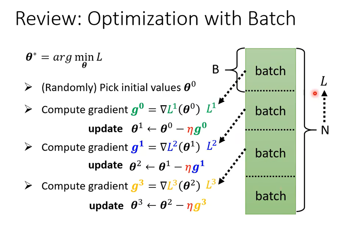
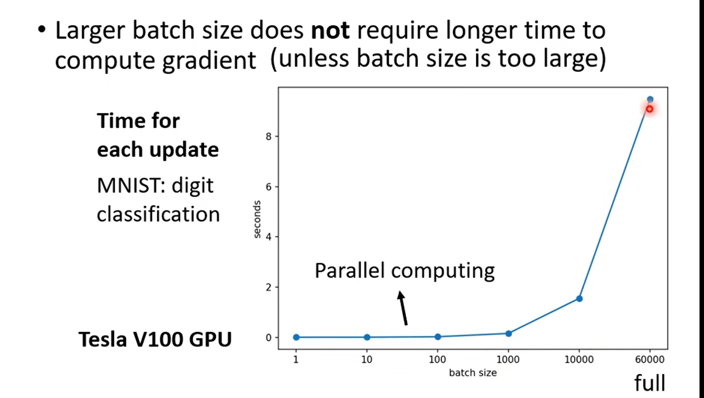
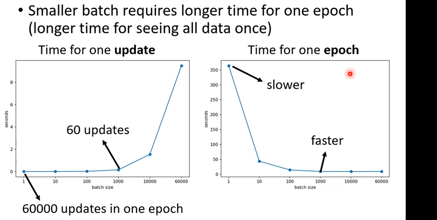
这里大家记得问自己一个问题:一个epoch 更新多少个参数?nums(batch)* parameters
例如,如果你有100个batch,那么在完成一个epoch后,每个参数会被更新100次。
shuffle :有可能batch结束后,就会重新分一次batch
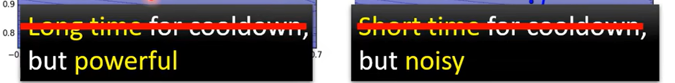
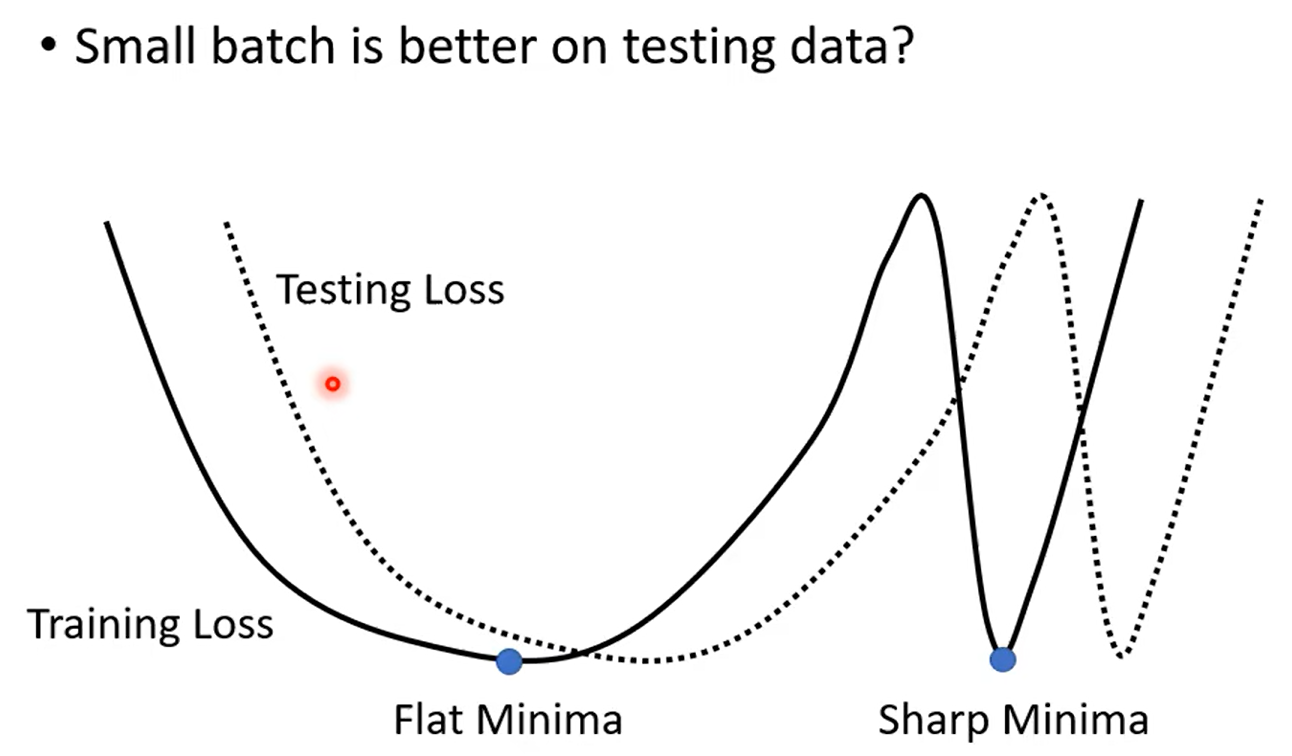
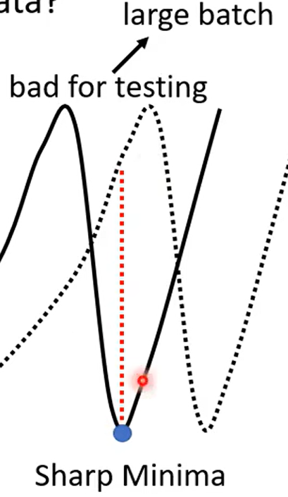
small vs big
这里举了两个极端的例子,也是我们常见的学习方法:取极限看效果
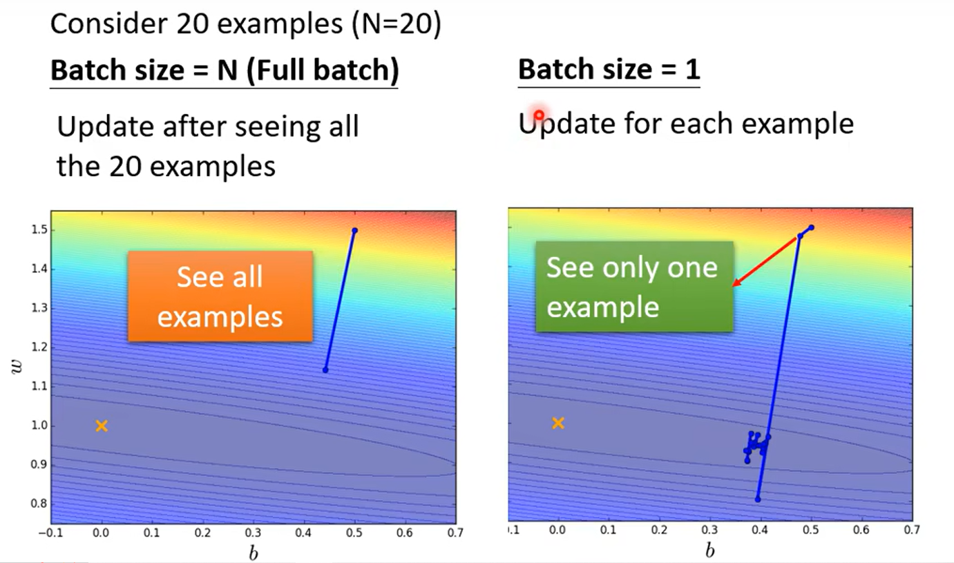
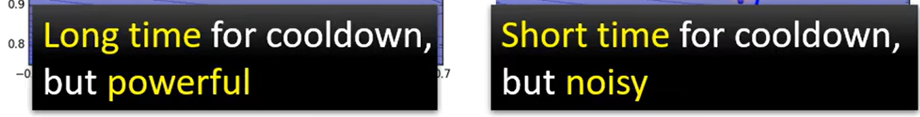
![image-20240411194814890](https://img-blog.csdnimg.cn/img_convert/8d750bd27a704731da2e279fbd9758d7.png)
未考虑平行运算(并行 --gpu)
![image-20240411195047480](https://img-blog.csdnimg.cn/img_convert/3ff59782843d9e769007e2cee1e4883b.png)
![image-20240411195201626](https://img-blog.csdnimg.cn/img_convert/c0f960522eec60ea4842bbf33a91d6d0.png)
![image-20240411195334111](https://img-blog.csdnimg.cn/img_convert/26c293073ba172a5389685306120e3c5.png)
![image-20240411195439085](https://img-blog.csdnimg.cn/img_convert/2f7fd5d562deac8fd88abc5ea5268637.png)
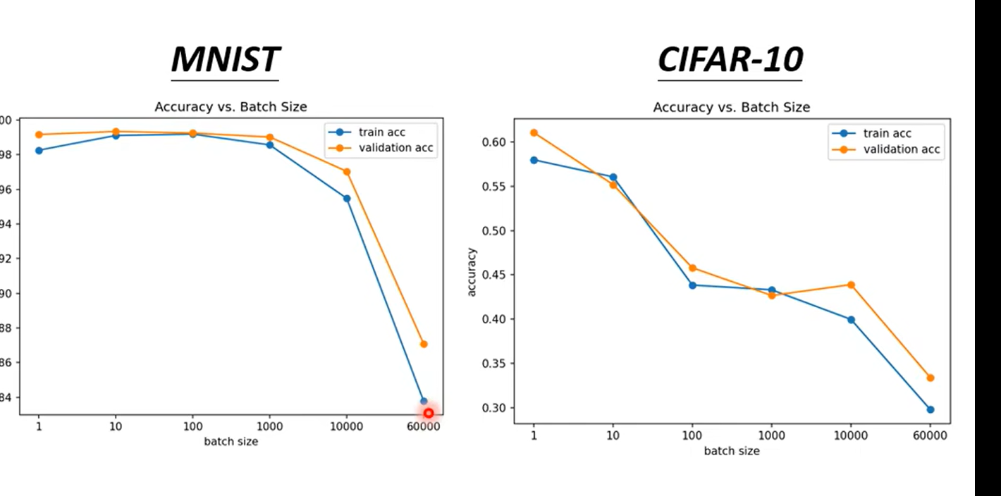
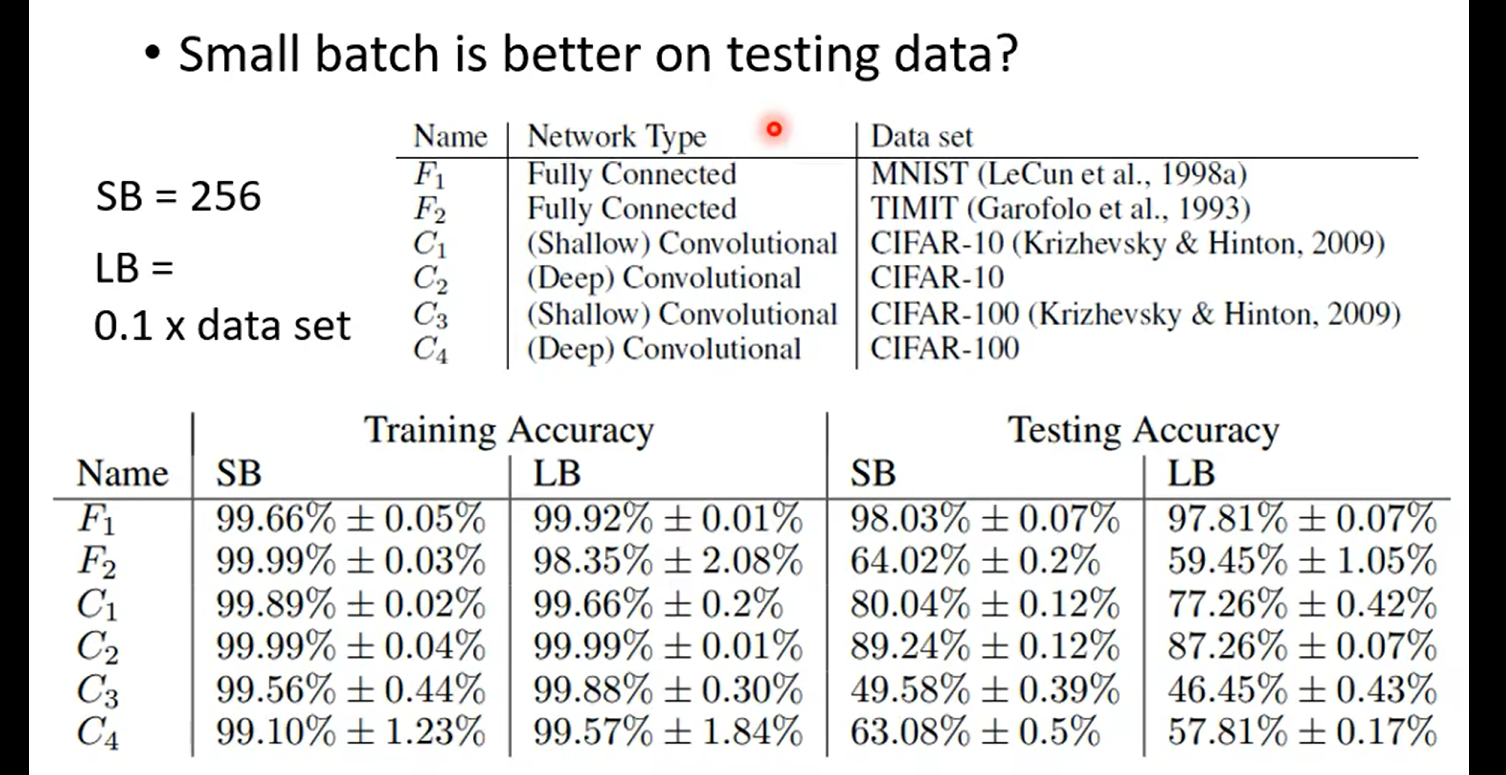
over fitting: 比较train 和test
![image-20240411195730628](https://img-blog.csdnimg.cn/img_convert/cb7c1809d2b1ea7da2cfdc4846016fc0.png)
![image-20240411195807268](https://img-blog.csdnimg.cn/img_convert/db5dbaad30305f1879015714e659f47e.png)
Aspect | Small Batch Size(100个样本) | Large Batch Size(10000个样本) |
---|---|---|
Speed for one update (no parallel) | Faster | Slower |
Speed for one update (with parallel) | Same | Same (not too large) |
Time for one epoch | Slower | Faster |
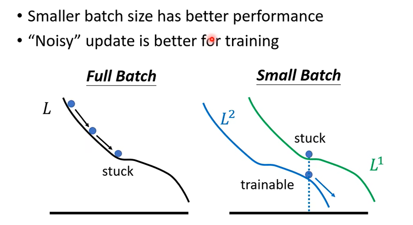
Gradient | Noisy | Stable |
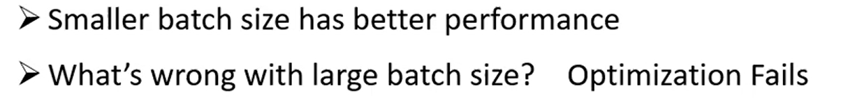
Optimization | Better | Worse |
Generalization | Better | Worse |
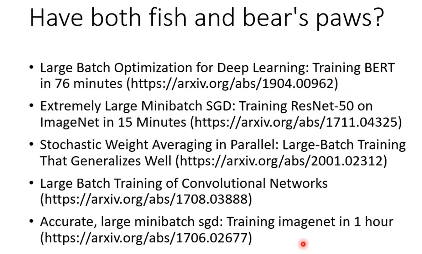
batch is a hyperparameter……
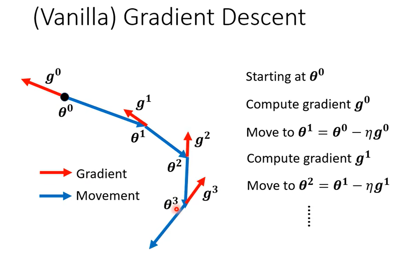
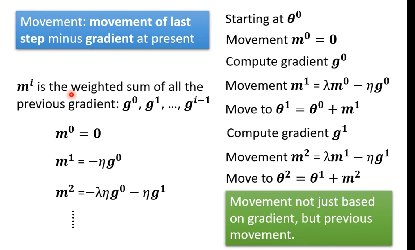
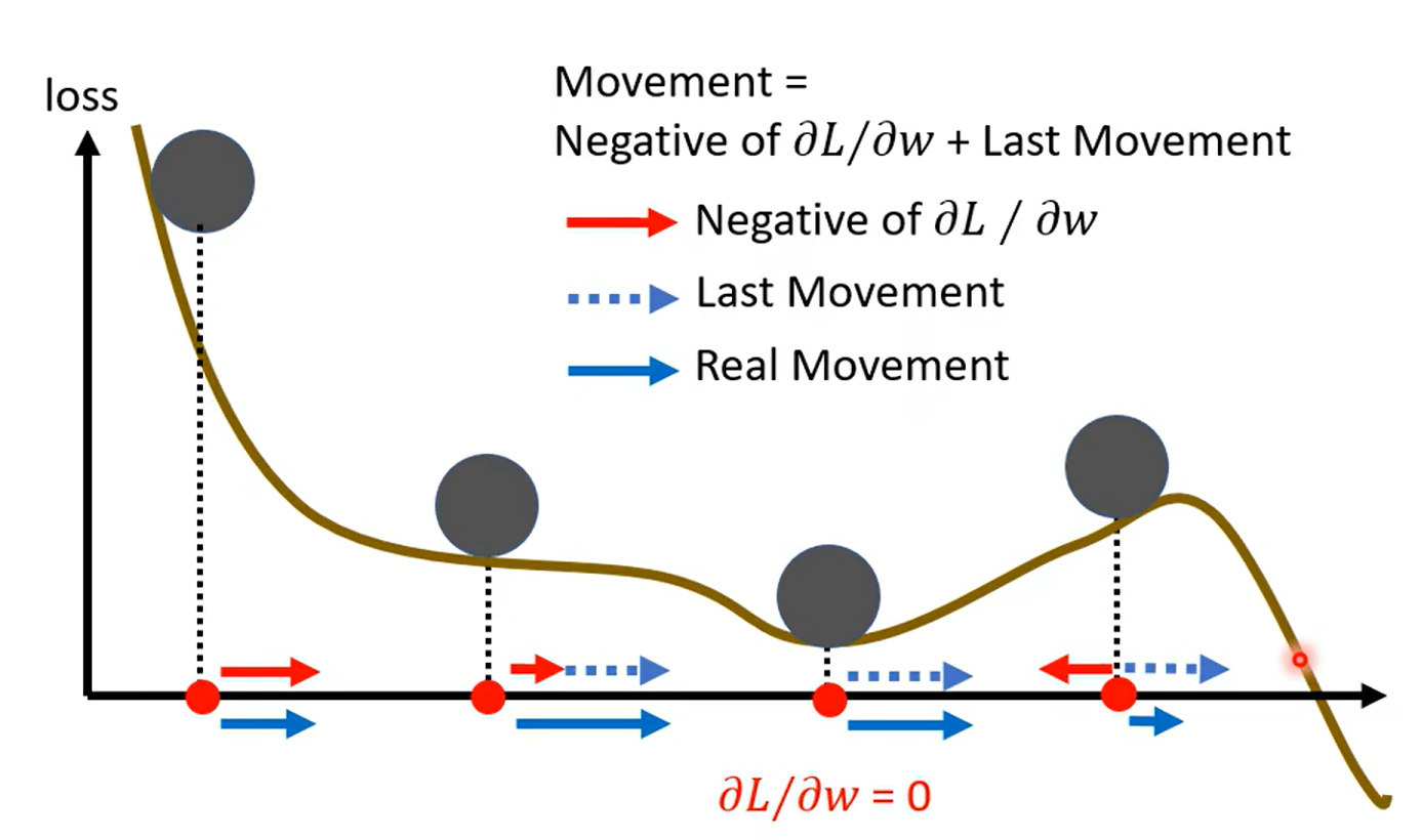
Momentum
惯性
![image-20240411200222463](https://img-blog.csdnimg.cn/img_convert/1cb42767e1f7faf0a9c625d64b55e84b.png)
![image-20240411200312757](https://img-blog.csdnimg.cn/img_convert/cdedd951048bbd3c99ab0f8786521417.png)
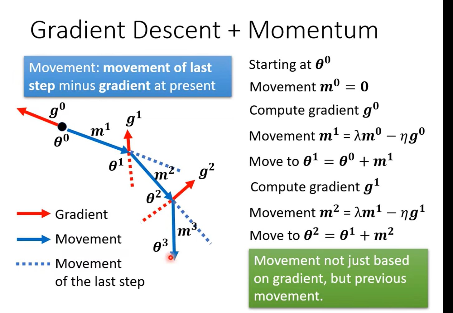
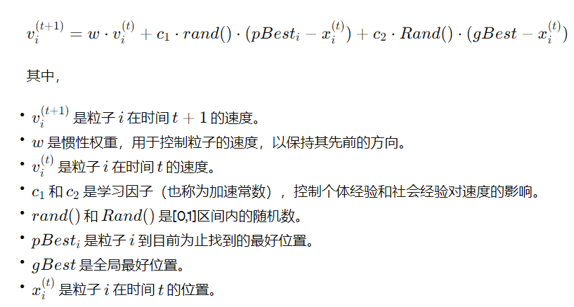
知道学到这里想到什么嘛……粒子群算法的公式不知道你们有没有了解,看下面那个w*vi 有没有感觉这种思想还挺常见的,用来做局部最小值的优化的
![image-20240411201955070](https://img-blog.csdnimg.cn/img_convert/3004d19c18b8a4330d77ecb4562aa65a.png)
![image-20240411202039014](https://img-blog.csdnimg.cn/img_convert/4024409f8ef25631f35520174961c88c.png)